Bobby Durrett's DBA Blog

This is a follow up to my July post. I have had almost two months to work with my new Selectloop Python script and I want to tell people what I learned so it will be helpful to them. Also it will help me to write this out and think about what I want to say.

First, I want to say that even though this post is about AI it is not generated by AI. This is all my words. I’m not even going to use spell or grammar checkers. I tend to write without commas so unless I get motivated to go back later and figure out where they go this may be comma free. I wrote my previous post but I did go to Copilot for advice and I feel like it makes what I write more generic. With all the “AI slop” out there you don’t need me adding to it.

Second, I was very suprised at how little interest my previous post generated. I documented Selectloop both on this blog and internally. My own DBA team had zero interest and no one commented on the blog post and it did not get many hits. That’s fine but what is funny is how excited I am about Selectloop and what I learned through it. Somehow I have not connected with people about how significant this is. Maybe it is because I have been on this AI journey and many of my readers and coworkers have not. Maybe people have been burned out on too much AI hype. To finally find a valuable use for AI has been such a joy. Maybe this post will help. I’ve learned some practical things:

• Run Selectloop for only a few minutes and look for quick results
• The generated queries are often more useful than the final report
• If you ask the same question twice it might give a good answer once and a bad the other time

So, I’ve simplified the command line to look like this:

python selectloop.py MYDATABASE question.txt

It runs with these settings:

• 30 select statements
• 120 second timeout for SQL query and AI inference
• 5000 line max rows fetched from query

This typically runs in a few minutes. I like to set it running while doing something else. You can also run several runs at the same time. 30 queries is enough to see if it is going down the right path. This is just from my experience. Sometimes the queries have syntax errors so you want to run enough so you get a fair number that actually run.

Here is an example of a simple question.txt file:

Find the top query for the past week and
describe its plan and purpose if you can.

Here is the console output from the run:

$ python selectloop.py MYDATABASE question.txt

Database: MYDATABASE
Question file: question.txt
Report file: selectloop_report_07482b1e.txt
Number of loops: 30
Query and Bedrock timeout in seconds: 120
Maximum number of rows fetched from query: 5000

Processing select statement 1 prompt length = 355
Processing select statement 2 prompt length = 1321
Processing select statement 3 prompt length = 1789
Processing select statement 4 prompt length = 2958
Processing select statement 5 prompt length = 5237
Processing select statement 6 prompt length = 6721
Processing select statement 7 prompt length = 8025
Processing select statement 8 prompt length = 9642
Processing select statement 9 prompt length = 10419
Processing select statement 10 prompt length = 10853
Processing select statement 11 prompt length = 11463
Processing select statement 12 prompt length = 14170
Processing select statement 13 prompt length = 14706
Processing select statement 14 prompt length = 15017
Processing select statement 15 prompt length = 15485
Processing select statement 16 prompt length = 15935
Processing select statement 17 prompt length = 17948
Processing select statement 18 prompt length = 21775
Processing select statement 19 prompt length = 23310
Processing select statement 20 prompt length = 24142
Processing select statement 21 prompt length = 26078
Processing select statement 22 prompt length = 34193
Processing select statement 23 prompt length = 36095
Processing select statement 24 prompt length = 36933
Processing select statement 25 prompt length = 37713
Processing select statement 26 prompt length = 43045
Processing select statement 27 prompt length = 49334
Processing select statement 28 prompt length = 51252
Processing select statement 29 prompt length = 54094
Processing select statement 30 prompt length = 55196

Generating final report

Run time in seconds: 179

Here is the final report.

*** Report generated by AI. It may contain errors. ***

TOP QUERY REPORT: PAST WEEK
===========================================================================

MOST EXECUTED QUERY (SELECT 3)
-------------------------------
SQL ID : d7bgf84kwj3s7
Executions : 2,816,949
Last Active : 2026-09-29 22:02:38

SQL Text:
  SELECT /*+ OPT_PARAM('_parallel_syspls_obey_force' 'false') */
  P.VALCHAR FROM SYS.OPTSTAT_USER_PREFS$ P
  WHERE P.OBJ#=:B2 AND P.PNAME=:B1

PURPOSE:
This is an internal Oracle optimizer statistics query. It reads
per-object optimizer preferences from the SYS.OPTSTAT_USER_PREFS$
table. Oracle calls it during statistics gathering to check whether
any object-level overrides (e.g. degree, method_opt) have been set
via DBMS_STATS.SET_TABLE_PREFS.

EXECUTION PLAN (SELECT 4):
  Step 0: SELECT STATEMENT (cost=1)
  Step 1: TABLE ACCESS BY INDEX ROWID on SYS.OPTSTAT_USER_PREFS$
  Step 2: INDEX UNIQUE SCAN on SYS.I_USER_PREFS$
          Access: P.OBJ#=:B2 AND P.PNAME=:B1

The plan is optimal: a unique index lookup with no disk reads
(SELECT 5: disk_reads=0) and exactly 1 buffer get per execution.
Avg elapsed and CPU times are near zero microseconds per call.

CONTEXT (SELECT 6, 7, 11):
The single ASH sample ties this SQL to SYS running DBMS_SCHEDULER
job ORA$AT_OS_OPT_SY_13592, the Oracle auto optimizer stats task.
SELECT 11 confirms "auto optimizer stats collection" is ENABLED and
completing successfully across daily maintenance windows (SELECT 16).

No action is required. This is expected Oracle background activity.
===========================================================================

This was not an active database so the top query was a system generated one.

Notice how it refers to the select numbers like this:

EXECUTION PLAN (SELECT 4):
  Step 0: SELECT STATEMENT (cost=1)
  Step 1: TABLE ACCESS BY INDEX ROWID on SYS.OPTSTAT_USER_PREFS$
  Step 2: INDEX UNIQUE SCAN on SYS.I_USER_PREFS$
          Access: P.OBJ#=:B2 AND P.PNAME=:B1

Here is select number 4:

-- SELECT number 4

-- Retrieves execution plan details for SQL ID 'd7bgf84kwj3s7' from v$sql_plan.

SELECT
    p.plan_hash_value,
    p.operation,
    p.options,
    p.object_owner,
    p.object_name,
    p.object_type,
    p.cost,
    p.cardinality,
    p.bytes,
    p.cpu_cost,
    p.io_cost,
    p.access_predicates,
    p.filter_predicates,
    p.id,
    p.parent_id,
    p.depth,
    p.position
FROM v$sql_plan p
WHERE p.sql_id = 'd7bgf84kwj3s7'
ORDER BY p.plan_hash_value, p.id;

PLAN_HASH_VALUE        OPERATION        OPTIONS OBJECT_OWNER         OBJECT_NAME    OBJECT_TYPE COST CARDINALITY BYTES CPU_COST IO_COST                  ACCESS_PREDICATES FILTER_PREDICATES ID PARENT_ID DEPTH POSITION 
--------------- ---------------- -------------- ------------ ------------------- -------------- ---- ----------- ----- -------- ------- ---------------------------------- ----------------- -- --------- ----- -------- 
      324713838 SELECT STATEMENT           None         None                None           None    1        None  None     None    None                               None              None  0      None     0        1 
      324713838 SELECT STATEMENT           None         None                None           None    1        None  None     None    None                               None              None  0      None     0        1 
      324713838     TABLE ACCESS BY INDEX ROWID          SYS OPTSTAT_USER_PREFS$          TABLE    1           1    42     8381       1                               None              None  1         0     1        1 
      324713838     TABLE ACCESS BY INDEX ROWID          SYS OPTSTAT_USER_PREFS$          TABLE    1           1    42     8381       1                               None              None  1         0     1        1 
      324713838            INDEX    UNIQUE SCAN          SYS       I_USER_PREFS$ INDEX (UNIQUE)    0           1  None     1050       0 "P"."OBJ#"=:B2 AND "P"."PNAME"=:B1              None  2         1     2        1 
      324713838            INDEX    UNIQUE SCAN          SYS       I_USER_PREFS$ INDEX (UNIQUE)    0           1  None     1050       0 "P"."OBJ#"=:B2 AND "P"."PNAME"=:B1              None  2         1     2        1 

6 rows selected.

Elapsed time: 0.00 seconds

It’s really easy to refer back to the select statements from the final report using the number.

I’ve updated the repository to contain this updated version: https://github.com/bobbydurrett/SelectLoop

The only hassle with the repository is that you have to do your own setup of your AWS account and database credentials. But the main code is all there in selectloop.py.

So, the point of this is just that Selectloop will run 30 queries for you against an Oracle database. You can ask it whatever you want. It runs for a few minutes. It may or may not be useful. But there have been times when it has been very useful in my work. You really have nothing to lose cutting one or more executions of Selectloop loose while you continue to work in other ways. Chances are if it is useful you will find not only good information in the final report, but also in the list of select statements and their output. I don’t know. I think it is extremely cool. If you are up for it, give it a try.

Bobby

Introduction

This post describes a way to use a Large Language Model (LLM) to investigate Oracle database problems. In this approach, the LLM repeatedly generates SELECT statements based on previous queries and their results. Each query provides additional context, allowing the LLM to gather information step by step before producing a final report for a DBA to review.

My previous attempts at using an LLM only performed a single inference. I had to gather the input data myself and decide what output I wanted the LLM to produce. In the SELECT Loop approach the LLM can gather its own information through each query it generates. Every iteration expands the context available to the model, allowing it to investigate a problem in several steps instead of trying to answer immediately with incomplete information.

Here is the outline of how this approach works:

1. Question -> LLM -> SELECT1 -> Oracle -> Output1
2. Question + SELECT1 + Output1 -> LLM -> SELECT2 -> Oracle -> Output2
3. Loop N times
4. Question + SELECT1 + Output1 + … + SELECTN + OutputN -> LLM -> Report
5. Report -> DBA

Question -> LLM -> SELECT1 -> Oracle -> Output1

The first step is to have the LLM generate a SQL query to try to answer some question about the database and then run it. The LLM’s prompt might look like this:

On an Oracle 11.2.0.4 database I want to investigate the performance of a sql statement with SQL_ID b4rj0h8hh0sxf.
Please generate a select statement that will give more information about b4rj0h8hh0sxf's performance.
Please only generate ASCII text.
Please keep to no more than 80 character lines.
Please output only the select statement that you want to run next.

The LLM generates some useful query against the database’s DBA or V$ views like:

SELECT
...
    s.iowait_delta           AS iowait_usecs,
    s.clwait_delta           AS clwait_usecs,
    s.apwait_delta           AS apwait_usecs,
    s.ccwait_delta           AS ccwait_usecs
FROM
    dba_hist_sqlstat   s
    JOIN dba_hist_snapshot sn
        ON  sn.snap_id     = s.snap_id
        AND sn.dbid        = s.dbid
        AND sn.instance_number = s.instance_number
WHERE
    s.sql_id = 'b4rj0h8hh0sxf'
    AND s.dbid = (SELECT dbid FROM v$database)
ORDER BY
    sn.begin_interval_time,
    s.plan_hash_value;

The next step is just to run the generated query against the database and get its output like:

   SNAP_ID BEGIN_TIME      END_TIME        PLAN_HASH_VALUE      EXECS  
---------- --------------- --------------- --------------- ----------
     88771 15-MAY-26 01:00 15-MAY-26 02:00      3752201481      11225
     88772 15-MAY-26 02:00 15-MAY-26 03:00      3752201481      22707
     88773 15-MAY-26 03:00 15-MAY-26 04:00      3752201481      11381
     88795 16-MAY-26 01:00 16-MAY-26 02:00      3752201481      11316
     88796 16-MAY-26 02:00 16-MAY-26 03:00      3752201481      23920
     88797 16-MAY-26 03:00 16-MAY-26 04:00      3752201481      10076
     88819 17-MAY-26 01:00 17-MAY-26 02:00      3752201481      11315
     88820 17-MAY-26 02:00 17-MAY-26 03:00      3752201481      24907
     88821 17-MAY-26 03:00 17-MAY-26 04:00      3752201481       9086
     88843 18-MAY-26 01:00 18-MAY-26 02:00      3752201481      11209
     88844 18-MAY-26 02:00 18-MAY-26 03:00      3752201481      24009
     88845 18-MAY-26 03:00 18-MAY-26 04:00      3752201481      10075

Question + SELECT1 + Output1 -> LLM -> SELECT2 -> Oracle -> Output2

Next take the original question and append the first SELECT statement and its output and request a second SELECT statement. The LLM suggested SELECT1. Now we are giving it both its SELECT1 query and its output. Then the LLM gets to take the next step in the problem investigation by generating a second SELECT statement. By showing it what it previously chose and the query output we are giving the LLM context that it didn’t have the first time we asked it the question. This prompt looks something like this:

On an Oracle 11.2.0.4 database I want to investigate the performance of a sql statement with SQL_ID b4rj0h8hh0sxf.
Following this prompt are the outputs of select statements that you recommended running. After evaluating them
please generate an additional select statement that will give more information about b4rj0h8hh0sxf's performance.
Please only generate ASCII text.
Please keep to no more than 80 character lines.
Please output only the select statement that you want to run next.
Output of your previous select statements:

This prompt would be followed by the first select statement and its output. I’m assuming that the output contains the SELECT statement and the query results. The query the LLM returns will probably be different from the first one because it already knows the result of the first query.

Once the LLM generates it, run the second query.

Loop N times

Now pass the original question plus all the queries and their outputs into the LLM requesting another SQL. Repeat this process N times. This pattern is the main point of this post. The LLM starts with the original question and generates a select statement. We run the query, append the query and its output to the prompt, and ask for another query. This process repeats until we have gathered enough information. The LLM is taking us down its own path investigating the question.

Keep generating new SELECT statements based on all the previous SELECT statements and their outputs.

Question + SELECT1 + Output1 + … + SELECTN + OutputN -> LLM -> Report

Finally stop generating new queries and take all the ones you have generated and all their outputs and ask the LLM to generate a final report. Here is part of a report:

## 4. The Plan Change Event on 26-JUN-26

On snap 89780 (26-JUN-26 02:00-03:00) plan 361274665 appeared for
35 executions alongside the normal plan. By snap 89781 (03:00-04:00)
the bad plan had taken over entirely.

Performance comparison for 26-JUN-26:

| Metric           | Normal plan  | Bad plan snap89781 | Bad plan snap89782 |
|------------------|-----------   |---------------------|---------------------|
| Executions       | 16,775 (03h) | 11                  | 13                  |
| Avg elapsed (s)  | 0.08         | 54.79               | 59.56               |
| Avg buffer gets  | 17,673       | 14,982,688          | 18,208,586          |
| Avg disk reads   | 37           | 6,832               | 6,463               |
| Avg I/O wait (s) | ~0           | 3.31                | 3.78                |
| Rows returned    | ~155         | ~73,765/exec        | ~72,639/exec        |

The bad plan is approximately **500x slower** per execution and
performs **800-1,000x more buffer gets**. Disk reads per execution
jump from ~37 to ~6,800.

What makes this interesting is that the LLM chose the sequence of queries that gathered the information used in this report.

Report -> DBA

The last step is for the DBA to review the report. No one should look at an AI generated report like this and act on it without an experienced DBA reviewing it. I don’t see this kind of report replacing DBAs. I see it as empowering them. Instead of me manually writing and running various queries to solve a problem I can give the problem to an LLM to take a first crack at it.

Conclusion

I struggled to find a practical use for LLMs in my DBA work until I started experimenting with this SELECT loop approach. By repeatedly generating queries, evaluating their results, and using that information to drive the next query, the LLM can investigate a problem before producing a final report. I don’t see this replacing DBAs, but I do see it helping experienced DBAs investigate problems more quickly.

P.S. I uploaded the sample code to a Github repository if you want to run it: https://github.com/bobbydurrett/SelectLoop

DBAs spend a lot of time reviewing reports about the health of their databases. I’ve used an LLM to speed up that process.

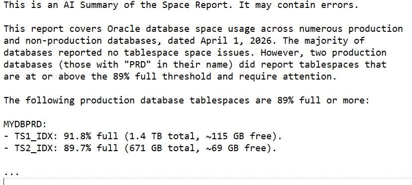
I took a daily report about our Oracle databases and used an LLM to generate a short summary that lets a DBA immediately see which databases need attention.

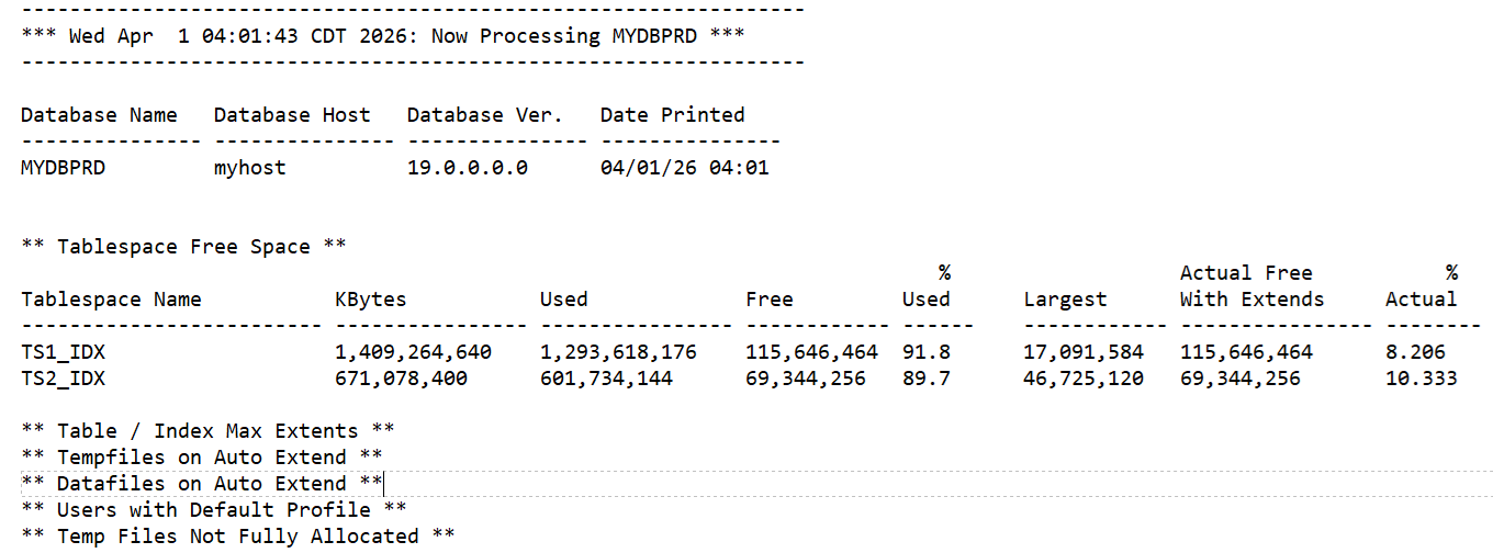
A typical report looks like this for each database:

The full report has over 2,000 lines that must be manually scanned by the on-call DBA each day.

The LLM-generated summary looks like this:

This summary immediately shows which databases need attention. We still manually scan the entire report but having the summary in the body of the email (with the full report attached) lets us see at a quick glance what needs attention and how urgent it is. The summary does not replace the full report; it only highlights the items that are most likely to be important. In our environment we chose 89% full as the point where we start reporting on space issues.

I’m using AWS Bedrock with the Claude Sonnet 4.6 model. Here is the Python
function that sends the combined prompt and report to Bedrock and returns the summary:

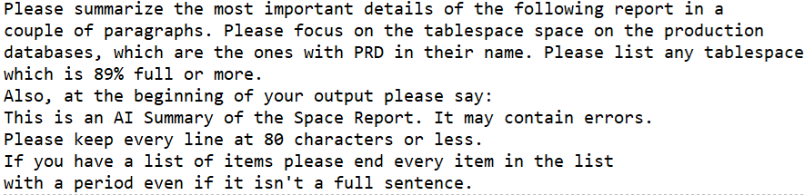
Here is the prompt that preceeds the report:

This simple use of an LLM has saved me time by putting a quick summary in the email body while preserving the full report for detailed review.

Bobby

I am working on an Oracle 19c database running on a RHEL 7 VM. I have been trying to roll back this patch:

Patch 30763851 IMPDP 11.2 TO 18C OR HIGHER HITS ORA-904 WHEN TABLES HAVE EXTENDED STATISTICS

I have it sitting on top of 19.5

Database Release Update: 19.5.0.0.191015 (30125133)

The Opatch rollback command ran fine, but Datapatch threw these errors:

[2025-10-22 18:50:15]   -> Error at line 11329: script rdbms/admin/dpload.sql
[2025-10-22 18:50:15]       - ORA-04063: view "SYS.KU$_OPQTYPE_VIEW" has errors"
[2025-10-22 18:50:15]   -> Error at line 11331: script rdbms/admin/dpload.sql
[2025-10-22 18:50:15]       - ORA-04063: view "SYS.KU$_OPQTYPE_VIEW" has errors"
[2025-10-22 18:50:15]   -> Error at line 11333: script rdbms/admin/dpload.sql
[2025-10-22 18:50:15]       - ORA-04063: view "SYS.KU$_OPQTYPE_VIEW" has errors"
[2025-10-22 18:50:15]   -> Error at line 11335: script rdbms/admin/dpload.sql
[2025-10-22 18:50:15]       - ORA-04063: view "SYS.KU$_OPQTYPE_VIEW" has errors"
[2025-10-22 18:50:15]   -> Error at line 11337: script rdbms/admin/dpload.sql
[2025-10-22 18:50:15]       - ORA-04063: view "SYS.KU$_OPQTYPE_VIEW" has errors"
[2025-10-22 18:50:15]   -> Error at line 11339: script rdbms/admin/dpload.sql
[2025-10-22 18:50:15]       - ORA-04063: view "SYS.KU$_OPQTYPE_VIEW" has errors"
[2025-10-22 18:50:15]   -> Error at line 11341: script rdbms/admin/dpload.sql
[2025-10-22 18:50:15]       - ORA-04063: view "SYS.KU$_OPQTYPE_VIEW" has errors"
[2025-10-22 18:50:15]   -> Error at line 11343: script rdbms/admin/dpload.sql
[2025-10-22 18:50:15]       - ORA-04063: view "SYS.KU$_OPQTYPE_VIEW" has errors"
[2025-10-22 18:50:15]   -> Error at line 11355: script rdbms/admin/dpload.sql
[2025-10-22 18:50:15]       - ORA-04063: view "SYS.KU$_P2TPARTCOL_VIEW" has errors"
[2025-10-22 18:50:15]   -> Error at line 11357: script rdbms/admin/dpload.sql
[2025-10-22 18:50:15]       - ORA-04063: view "SYS.KU$_P2TPARTCOL_VIEW" has errors"
[2025-10-22 18:50:15]   -> Error at line 11363: script rdbms/admin/dpload.sql
[2025-10-22 18:50:15]       - ORA-04063: view "SYS.KU$_SP2TPARTCOL_VIEW" has errors"
[2025-10-22 18:50:15]   -> Error at line 11365: script rdbms/admin/dpload.sql
[2025-10-22 18:50:15]       - ORA-04063: view "SYS.KU$_SP2TPARTCOL_VIEW" has errors"
[2025-10-22 18:50:15]   -> Error at line 11381: script rdbms/admin/dpload.sql
[2025-10-22 18:50:15]       - ORA-04063: view "SYS.KU$_COLUMN_VIEW" has errors"
[2025-10-22 18:50:15]   -> Error at line 11383: script rdbms/admin/dpload.sql
[2025-10-22 18:50:15]       - ORA-04063: view "SYS.KU$_COLUMN_VIEW" has errors"
[2025-10-22 18:50:15]   -> Error at line 11385: script rdbms/admin/dpload.sql
[2025-10-22 18:50:15]       - ORA-04063: view "SYS.KU$_COLUMN_VIEW" has errors"
[2025-10-22 18:50:15]   -> Error at line 11387: script rdbms/admin/dpload.sql
[2025-10-22 18:50:15]       - ORA-04063: view "SYS.KU$_COLUMN_VIEW" has errors"
[2025-10-22 18:50:15]   -> Error at line 11389: script rdbms/admin/dpload.sql
[2025-10-22 18:50:15]       - ORA-04063: view "SYS.KU$_PCOLUMN_VIEW" has errors"
[2025-10-22 18:50:15]   -> Error at line 11391: script rdbms/admin/dpload.sql
[2025-10-22 18:50:15]       - ORA-04063: view "SYS.KU$_PCOLUMN_VIEW" has errors"
[2025-10-22 18:50:15]   -> Error at line 11393: script rdbms/admin/dpload.sql
[2025-10-22 18:50:15]       - ORA-04063: view "SYS.KU$_PCOLUMN_VIEW" has errors"
[2025-10-22 18:50:15]   -> Error at line 11395: script rdbms/admin/dpload.sql
[2025-10-22 18:50:15]       - ORA-04063: view "SYS.KU$_PCOLUMN_VIEW" has errors"
[2025-10-22 18:50:15]   -> Error at line 11397: script rdbms/admin/dpload.sql
[2025-10-22 18:50:15]       - ORA-04063: view "SYS.KU$_P2TCOLUMN_VIEW" has errors"
[2025-10-22 18:50:15]   -> Error at line 11399: script rdbms/admin/dpload.sql
[2025-10-22 18:50:15]       - ORA-04063: view "SYS.KU$_P2TCOLUMN_VIEW" has errors"
[2025-10-22 18:50:15]   -> Error at line 11401: script rdbms/admin/dpload.sql
[2025-10-22 18:50:15]       - ORA-04063: view "SYS.KU$_SP2TCOLUMN_VIEW" has errors"
[2025-10-22 18:50:15]   -> Error at line 11403: script rdbms/admin/dpload.sql
[2025-10-22 18:50:15]       - ORA-04063: view "SYS.KU$_SP2TCOLUMN_VIEW" has errors"
[2025-10-22 18:50:15]   -> Error at line 11405: script rdbms/admin/dpload.sql
[2025-10-22 18:50:15]       - ORA-04063: view "SYS.KU$_COLUMN_VIEW" has errors"
[2025-10-22 18:50:15]   -> Error at line 11407: script rdbms/admin/dpload.sql
[2025-10-22 18:50:15]       - ORA-04063: view "SYS.KU$_COLUMN_VIEW" has errors"
[2025-10-22 18:50:15]   -> Error at line 11409: script rdbms/admin/dpload.sql
[2025-10-22 18:50:15]       - ORA-04063: view "SYS.KU$_PCOLUMN_VIEW" has errors"
[2025-10-22 18:50:15]   -> Error at line 11411: script rdbms/admin/dpload.sql
[2025-10-22 18:50:15]       - ORA-04063: view "SYS.KU$_PCOLUMN_VIEW" has errors"

I checked DBA_OBJECTS, and all the SYS objects are VALID. I tried querying one of the views and it worked fine. So, I went to My Oracle Support, our Oracle database support site, and searched for ORA-04063 and one of the view names and found nothing. A Google search also came up empty. I tried just ignoring it but that didn’t work. My whole goal in doing this was to apply the October 2025 patches that just came out this week. But because the SQL patch registry indicated that patch 30763851 rolled back with errors, every time I applied a new patch it would try to roll 30763851 back first and error again. Here is what DBA_REGISTRY_SQLPATCH looked like after two failed rollback attempts:

INSTALL_ID   PATCH_ID PATCH_TYPE ACTION          STATUS        
---------- ---------- ---------- --------------- --------------
         1   30125133 RU         APPLY           SUCCESS       
         2   30763851 INTERIM    APPLY           SUCCESS       
         3   30763851 INTERIM    ROLLBACK        WITH ERRORS   
         3   30763851 INTERIM    ROLLBACK        WITH ERRORS   
         4   30763851 INTERIM    ROLLBACK        WITH ERRORS   
         4   30763851 INTERIM    ROLLBACK        WITH ERRORS   

Each rollback attempt tried twice so I have four failures with two rollback attempts.

I opened a case with Oracle support just in case this was a known issue that wasn’t available for me to find on my own. Sometimes that happens. But while waiting on Oracle I kept trying to fix it myself.

The errors refer to $ORACLE_HOME/rdbms/admin/dpload.sql which I think reloads datapump after some change. It runs catmetviews.sql and catmetviews_mig.sql which have the CREATE VIEW statements for the views getting errors, like SYS.KU$_OPQTYPE_VIEW. But the code in catmetviews_mig.sql wasn’t straightforward. I imagined running some sort of trace to see why the script was throwing the ORA-04063 errors, but I never had to take it that far.

At first all this stressed me out. I thought, “I can’t back out this patch. I will never be able to patch this database to a current patch level.” Then I chilled out and realized that if it was a problem with Oracle’s code, they had to help me back out 30763851. But it might take some time to work through an SR with Oracle.

But what if it wasn’t an issue with Oracle’s code but something weird in our environment? I didn’t think it indicated a real problem, but there were some weird messages coming out that I am used to seeing. They were from triggers that come with an auditing tool called DB Protect. They were throwing messages like this:

[SYS.SENSOR_DDL_TRIGGER_A] Caught a standard exception: aliasId=100327, error=-29260, message="ORA-29260: network error: TNS:no listener"

We are used to seeing these errors when we do DDL but prior to this it didn’t cause any actual problems. We had already decommisioned the DB Protect tool but had not cleaned up the triggers. Dropping SYS.SENSOR_DDL_TRIGGER_A eliminated the ORA-04063 errors.

Probably no one will ever encounter this same issue, but I thought I would document it. If you have the same symptoms and you are not using DB Protect any more, do these commands:

DROP TRIGGER SYS.SENSOR_DDL_TRIGGER_A;
DROP TRIGGER SYS.SENSOR_DDL_TRIGGER_B;

I think the A trigger was the problem, but we don’t need either one.

Anyway, this post is just so someone who searches for ORA-04063 and one of the views will find this information and drop the triggers if they have them. It’s a long shot but might as well document it for posterity and for me.

Bobby

I recently migrated my WordPress blog from Amazon Linux 2 to Amazon Linux 2023 to take advantage of newer software versions. The process was mostly smooth, but I wanted to document a few things I ran into—especially around encryption setup.

I followed these instructions for setting WordPress up on AL 2023: https://docs.aws.amazon.com/linux/al2023/ug/hosting-wordpress-aml-2023.html

The first thing I had to do was follow these instructions to get Apache, PHP, and MariaDB setup: https://docs.aws.amazon.com/linux/al2023/ug/ec2-lamp-amazon-linux-2023.html

I also had to setup a new elastic ip: https://docs.aws.amazon.com/AWSEC2/latest/UserGuide/elastic-ip-addresses-eip.html

I used the security group that I had for my existing AL 2 EC2 so I had the right ip addresses opened up.

I copied the database over from the old to new EC2:

on the old server:

mysqldump -u blogdbuser -pMYPASSWORD --single-transaction --routines --triggers blogdb  > blogdb.sql

on the new server:

mysql -vvv -n -u blogdbuser -pMYPASSWORD blogdb <  blogdb.sql > blogdb.log

Similarly for the web pages and other files:

New server:

# clear out existing web server directory

cd /var/www/html

sudo rm -fr *

sudo rm -f .htaccess .user.ini .wpcli

Old server:

sudo tar -cvf /home/ec2-user/html.tar /var/www/html

New server:

sudo tar -xvf /home/ec2-user/html.tar -C /

Moving the DNS entries over to the new elastic ip address was easy. I just had the change the “A” records for bobbydurrettdba.com and www.bobbydurrettdba.com in Route 53. First, I changed the TTL from one day to 10 minutes so my changes would propogate quickly while I messed with things. Later I set these back. One day was 86400 seconds. Ten minutes was 600 seconds.

The biggest challenge I had was getting encryption setup properly. The documentation missed a couple of key steps. I thought about just writing this post about the encryption part because it was the only thing that wasn’t straightforward.

I was following the steps in https://docs.aws.amazon.com/linux/al2023/ug/SSL-on-amazon-linux-2023.html and using the Let’s Encrypt script for getting certificates. This was called Certbot and documented here: https://eff-certbot.readthedocs.io/en/stable/install.html

There were two key things missing from this documentation:

• How to install Snap on Amazon Linux 2023
• The need for a port 80 VirtualHost

Certbot wants you to install something called Snap to use to install Certbot. I got this from a Google search:

sudo dnf install openssl mod_ssl

sudo wget -O /etc/yum.repos.d/snapd.repo https://bboozzoo.github.io/snapd-amazon-linux/al2023/snapd.repo

sudo dnf install snapd -y

sudo systemctl enable --now snapd.socket

sudo ln -s /var/lib/snapd/snap /snap

sudo reboot

The other undocumented thing was that I had to add these lines after the “Listen 80” line in /etc/httpd/conf/httpd.conf:

sudo vi /etc/httpd/conf/httpd.conf

after Listen 80 add this:

<VirtualHost *:80>
    DocumentRoot "/var/www/html"
    ServerName bobbydurrettdba.com
    ServerAlias www.bobbydurrettdba.com
</VirtualHost>

Then I just ran the documented Certbot commands like this:

sudo snap install --classic certbot

sudo ln -s /snap/bin/certbot /usr/bin/certbot

sudo certbot --apache

It took me a few iterations to get this right. Anyway, I just wanted to post a quick note documenting this.

Bobby

1. Introduction

I set out to use Machine Learning to monitor Oracle databases but ultimately chose not to. The most valuable lesson I learned was the importance of visualizing my data to determine the best approach. By examining real production performance issues, I developed scripts that trigger alerts during potential performance problems. I used six weeks of historical performance metrics to compare current behavior against past trends. I already knew that a high value for a given metric didn’t necessarily indicate a performance issue with business impact. In the end, I built a script that sends an alert when certain metrics are the top wait event and are performing three times worse than at any point in the past six weeks. While it doesn’t guarantee a business impact, it flags anomalies that are unusual enough to warrant investigation.

2. Why I Tried Machine Learning

I think anyone reading this post would know why I tried to use Machine Learning. It’s very popular now. I took a class online about ML with Python and I bought a book about the same subject. I had already used Python in some earlier classes and in my work, so it was natural to take a class/read a book about ML based on Python. As I mentioned in an earlier post, I studied AI in school many years ago and there have been many recent advances so naturally I wanted to catch up with the current state of the art in AI and ML. Having taken the class, and later having read a book, I needed some application of what I learned to a valuable business problem. We had a couple of bad performance problems with our Oracle databases and our current monitoring didn’t catch them. So, I wanted to use ML – specifically with PyTorch in a Python script – to write a script that would have alerted on those performance problems.

3. Failed Attempt Number One – Autoencoder

In my first attempt to write a monitoring script, I worked with Copilot and ChatGPT to hack together a script using an autoencoder model. I queried a bunch of our databases and collected a list of all the wait events. My idea was to treat each wait as an input to the autoencoder. For each wait, I pulled the number of events and the total wait time over the past hour. I didn’t differentiate between foreground and background waits—I figured AI could sort that out. I also included DB time and DB CPU time. These were all deltas between two hourly snapshots, so the data represented CPU and waits for a given hour.

The concept behind the autoencoder was to compress these inputs into a smaller set of values and then reconstruct the original inputs. With six weeks of hourly snapshots, I trained the autoencoder on that historical data, assuming it represented “normal” behavior. The idea was that any new snapshot that couldn’t be accurately reconstructed by the model would be considered abnormal and trigger an alert.

I got the model fully running across more than 20 production databases. I tuned the threshold so it would have caught two recent known performance issues. But in practice, it didn’t work well. It mostly triggered alerts on weekends when backups were running and I/O times naturally spiked. It wasn’t catching real performance problems—it was just reacting to predictable noise.

Here is the PyTorch autoencoder model:

# Define the Autoencoder model
class TabularAutoencoder(nn.Module):
    def __init__(self, input_dim):
        super(TabularAutoencoder, self).__init__()
        # Encoder
        self.encoder = nn.Sequential(
            nn.Linear(input_dim, 64),  # Reduce dimensionality from input_dim to 64
            #nn.LayerNorm(64),  # Layer Normalization for stability
            nn.ReLU(True),
            nn.Dropout(0.2),   # Dropout for regularization
            nn.Linear(64, 32),  # Reduce to 32 dimensions
            nn.ReLU(True),
            nn.Linear(32, 16),  # Bottleneck layer (compressing to 16 dimensions)
        )
        # Decoder
        self.decoder = nn.Sequential(
            nn.Linear(16, 32),  # Expand back to 32 dimensions
            nn.ReLU(True),
            nn.Linear(32, 64),  # Expand to 64 dimensions
            #nn.LayerNorm(64),  # Layer Normalization for stability
            nn.ReLU(True),
            nn.Linear(64, input_dim),  # Expand back to original input dimension
         )

    def forward(self, x):
        x = self.encoder(x)
        x = self.decoder(x)
        return x

4. Failed Attempt Number Two – Binary Classification

Much more recently, I came back to using a PyTorch model to build an alerting script. I had spent some time learning about large language models and exploring how to apply GenAI to business problems, rather than working with these simpler ML models in PyTorch. But I decided to give it another try and see if I could fix the limitations I ran into with the autoencoder approach.

I didn’t really expect binary classification to work, but it’s the simplest kind of ML model, so I thought it was worth a shot. I selected a few snapshots that occurred during a severe performance problem on an important Oracle database. I labeled these as 1 (problem), and the rest as 0 (no problem). It was easy enough to train a model that correctly identified the problem snapshots during training and testing.

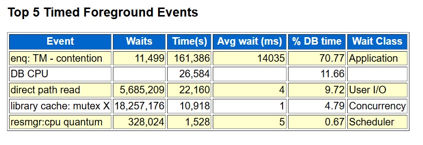
However, when I applied the model to later snapshots it hadn’t seen before, it started generating false alarms that didn’t make sense. It got even worse when I tried it on a completely different database. I had expected the model to pick up on the fact that the top wait event during the problem period was enq: TM – contention. A quick glance at the top foreground events in an AWR report made it obvious that this was the issue. But the trained model ended up sending an alert on snapshots that didn’t even have this wait event in the top waits.

Here is the PyTorch binary classification model:

"""

Mostly got the model from Copilot. input_dim is the number of performance
metrics which is over 100. Gets it down to 64 to 32 and then 1.
The ReLU functions add "non-linear" change to allow it to do
functions that the linear steps can't do.

"""
    
class MyModel(nn.Module):
    def __init__(self, input_dim):
        super(MyModel, self).__init__()
        self.fc1 = nn.Linear(input_dim, 64)
        self.relu1 = nn.ReLU()
        self.fc2 = nn.Linear(64, 32)
        self.relu2 = nn.ReLU()
        self.output = nn.Linear(32, 1)

    def forward(self, x):
        x = self.fc1(x)
        x = self.relu1(x)
        x = self.fc2(x)
        x = self.relu2(x)
        x = self.output(x)
        return x

Here are the foreground waits and cpu from an AWR report of the problem time:

5. Failed Attempt Number Three – Z-Score

While talking with Copilot, I decided to try a simple statistical approach to anomaly detection. One suggestion was to use a z-score. In my context, this meant looking at the top foreground wait event—enq: TM – contention—in the current snapshot and calculating its z-score relative to the mean and standard deviation of that wait’s values in previous snapshots.

Like the binary classification attempt, the z-score alerting script worked well with the original snapshots from the known problem period. But when I ran the same script against other databases, it produced a lot of false alarms.

Output of z-score script on problem database (alerts on expected snapshot):

   SNAP_ID SNAP_DTTIME         EVENT_NAME            RATIO_ZSCORE AVGWAIT_ZSCORE
---------- ------------------- --------------------- ------------ --------------
    151752 2025-06-19 00:00:41 enq: TM - contention     3.0878532     9.74301378

Output on another database (no rows expected):

   SNAP_ID SNAP_DTTIME         EVENT_NAME                    RATIO_ZSCORE AVGWAIT_ZSCORE
---------- ------------------- ----------------------------- ------------ --------------
     48916 2025-06-22 01:00:01 cursor: pin S wait on X         9.00654128     5.36254393
     48917 2025-06-22 02:00:06 cursor: pin S wait on X         7.16211659     8.09929239
     48918 2025-06-22 03:00:11 cursor: pin S wait on X         5.41578347     4.52106805
     48919 2025-06-22 04:00:13 cursor: pin S wait on X         4.69593403     4.08335551
     48920 2025-06-22 05:00:16 cursor: pin S wait on X         3.17592316     3.46979661
     49081 2025-06-28 22:00:32 cursor: pin S wait on X         4.62636243     3.15122436
     49254 2025-07-06 03:00:04 cursor: pin S wait on X         4.73771834     3.23654318
     49255 2025-07-06 04:00:10 cursor: pin S wait on X         3.96208561     3.61732606
     49289 2025-07-07 14:00:55 SQL*Net more data from dblink   18.2249941     6.61795927
     49364 2025-07-10 17:00:20 library cache lock              89.7469665     392.322777
     49365 2025-07-10 18:00:45 library cache lock              14.6228987      120.71596
     49760 2025-07-27 05:00:21 cursor: pin S wait on X         5.68469758     3.52381292

6. A Picture Is Worth a Thousand Words

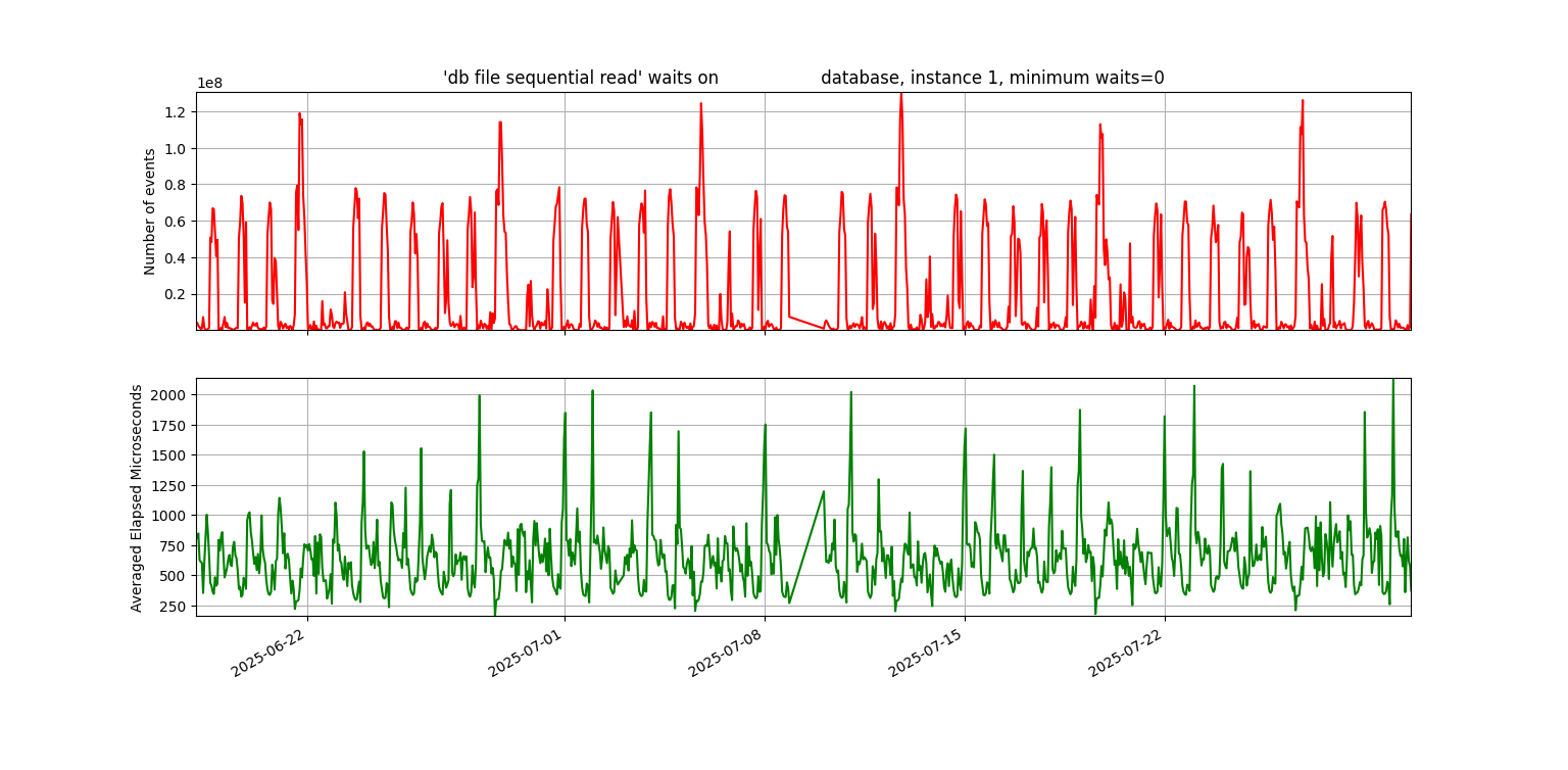
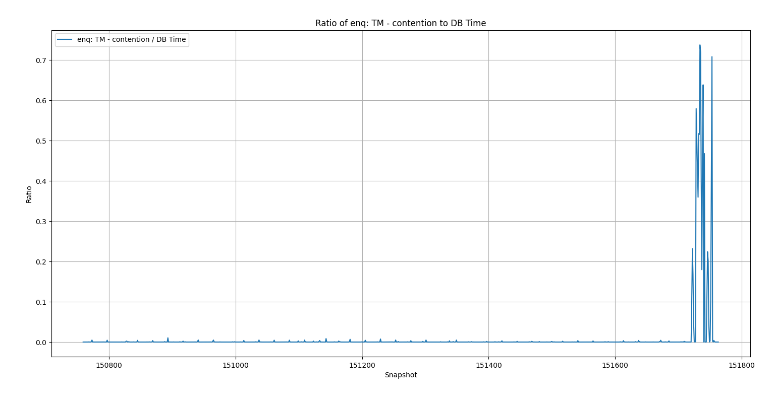
Now I’m getting to the high point of this post. I graphed the waits for the snapshots where the z-score worked and the ones where it didn’t—and the truth jumped out at me. In the database with the known problem, the graph of enq: TM – contention was almost a flat line across the bottom for six weeks, followed by a huge spike during the problem hours. In another database—or even the same one with a different top wait—the graph looked completely different: a wavy pattern, almost like a sine wave, stretching back across the entire six weeks.

“Heck!” I said to myself. “Why don’t I just look for top waits that are never close to this high in the past six weeks?” Sure, it might not always be a real business problem, but if a wait is so dramatically different from six weeks of history, it’s worth at least sending an email—if not a wake-up-in-the-middle-of-the-night page.

With z-score, we were sending an alert when a metric was three standard deviations from the mean. But for wavy waits like db file sequential read, that wasn’t selective enough. So, I designed a new monitoring script: it looks at the top wait in the snapshot, checks if it’s a higher percentage of DB time than CPU, and then compares it to the past six weeks. If it’s more than three times higher than it’s ever been in that history, it triggers an alert. This is all based on the percentage of total DB time.

First the wavy graph of db file sequential read waits:

Next, this is the key graph to this entire post. Not wavy:

The light clicked on when I saw this graph. The enq: TM – contention waits were insignificant until the problem occurred.

Here is the script that checks if we should alert: neveralert.sql

7. Don’t Check Your Brain at the Machine Learning Door

When I started with the autoencoder script, I felt overwhelmed—like many people do when first approaching Artificial Intelligence and Machine Learning. I expected the model to magically work without fully understanding how or why. I relied on chat tools to help me piece together code I didn’t grasp, and when it didn’t work, I couldn’t explain why. I’m trying to be honest about my journey here so it might help others and remind myself what I learned.

Each step—from binary classification to z-score to manual logic—brought me closer to a solution rooted in my own experience. You must use your own brain. This has always been true in Oracle performance work: you can’t just follow something you read or heard about without understanding it. You need to think critically and apply your domain knowledge.

If it sounds like I didn’t get anything out of my machine learning training, that’s not the case. Both the class and the book emphasized the importance of visualizing data to guide modeling decisions. They used Matplotlib to create insightful graphs, and while I’ve used simpler visualizations in my own PythonDBAGraphs repo, this experience showed me the value of going deeper with data visualization. I think both the class and book would agree: visualizing your data is one of the best ways to decide how to use it.

Even though this journey didn’t end with a PyTorch-based ML solution, it sharpened my understanding of both ML and Oracle performance—and I’m confident it will help me build better solutions in the future.

Bobby

Sunday four batch jobs that normally run in an hour had been stuck for 3 hours and had not completed the first unit of work out of many. Earlier in the day the on call DBA had applied a SQL Profile and cancelled the jobs and rerun them but it did not help. We picked a different SQL Profile, killed the jobs, and the jobs ran normally. How did we figure out the right plan to use for a SQL Profile?

The main clue came from the output of my sqlstat.sql script:

The good plan seemed to be 2367956558. EXECUTIONS_DELTA = 1 means that the SQL finished in that hour. Elapsed Average ms of 45177.105 was 45 seconds. 19790.066 was 19 seconds.

PLAN_HASH_VALUE END_INTERVAL_TIME         EXECUTIONS_DELTA Elapsed Average ms
--------------- ------------------------- ---------------- ------------------
     2367956558 20-APR-25 01.00.23.638 AM                1          45177.105
     2367956558 20-APR-25 03.00.29.921 AM                1          19790.066

The other plans 2166514251 and 3151484146 seemed to have executions that spanned multiple hours. For example, the first 2166514251 line had EXECUTIONS_DELTA = 0 which means it didn’t finish in that hour. Plus, the elapsed time of 8995202.39 ms = 8995 seconds = 2.5 hours suggests that it was running in parallel, probably for the entire hour.

PLAN_HASH_VALUE END_INTERVAL_TIME         EXECUTIONS_DELTA Elapsed Average ms
--------------- ------------------------- ---------------- ------------------
     2166514251 20-APR-25 01.00.23.638 AM                0         8995202.39

So, it seems clear that 2367956558 is the best plan.

I could say a lot more about this incident, but I wanted to focus on the sqlstat.sql output. The values of EXECUTIONS_DELTA and Elapsed Average ms are keys to identifying plans with the best behavior.

Bobby

Introduction

Everyone who has heard the old saying “a picture is worth a thousand words” appreciates its simple wisdom. With Oracle databases you have situations where a graph of the output of a SQL query is easier to understand than the standard text output. It’s helpful to have a simple way to graph Oracle data, and Python has widely used libraries that make it easy.

This post describes a Python script that graphs data from an Oracle database using the Matplotlib graphics library. The script uses three widely used Python libraries: cx_Oracle, NumPy, and Matplotlib. This post provides a simple and easily understood example that can be reused whenever someone needs to graph Oracle data. It is written as a straight-line program without any functions or error handling to keep it as short and readable as possible. It demonstrates the pattern of cx_Oracle -> NumPy -> Matplotlib and the use of Matplotlib’s object-oriented approach.

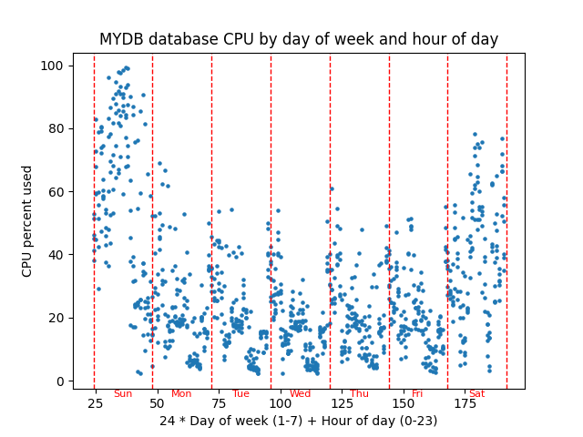
Here is an example graph:

The script graphs database server percent CPU used versus a combination of the day of week and the hour of the day to see if there is any pattern of CPU usage throughout a typical week. This graph has about 6 weeks of hourly AWR snapshots graphed in a scatter plot with CPU percentage on the Y axis and (24 * day of week) + hour of day as the X axis. You could think of the X axis as the hour of the week. This graph might be helpful in performance tuning because it shows whether CPU usage follows a weekly pattern.

Here is the current version of the script: scatter.py.

The script has three main parts which correspond to the three non-internal Python libraries that I use:

• cx_Oracle – Query the CPU data from an Oracle database
• NumPy – Massage query data to get it ready to be graphed
• Matplotlib – Graph the data

These libraries all have lots of great documentation, but Matplotlib’s documentation is confusing at first. At least it was for me. Here are three useful links:

Quick start – This is a great overview. The picture of the “Parts of a Figure” is helpful. I don’t know if earlier versions of Matplotlib had this picture.

Axes – This is a nice list of all the methods of an Axes object. Most of the code in the example script involves calling these methods. I have trouble finding these methods using a Google search, so I bookmarked this link.

Figure – The example script does not call any Figure object methods, but I wanted to document where to find them here. I bookmarked this URL as well as the Axes one because a Matplotlib graph is composed of at least one Figure and Axes object. With the Quick start link and these two lists of methods you have all you need to write Matplotlib scripts.

cx_Oracle

The query for this graph pulls operating system CPU metrics from the DBA_HIST_OSSTAT view and uses them to calculate the percent of the time the CPU is busy. It is made of two subqueries in a with statement and the final main query.

with
myoscpu as
(select
busy_v.SNAP_ID,
busy_v.VALUE BUSY_TIME,
idle_v.VALUE IDLE_TIME
from 
DBA_HIST_OSSTAT busy_v,
DBA_HIST_OSSTAT idle_v
where
busy_v.SNAP_ID = idle_v.SNAP_ID AND
busy_v.DBID = idle_v.DBID AND
busy_v.INSTANCE_NUMBER = idle_v.INSTANCE_NUMBER AND
busy_v.STAT_NAME = 'BUSY_TIME' AND
idle_v.STAT_NAME = 'IDLE_TIME'),

The myoscpu subquery pulls the CPU busy and idle times from the view along with the snapshot id. I think these are totals since the database last came up, so you have to take the difference between their values at two different points in time to get the CPU usage for that time.

myoscpudiff as
(select
after.SNAP_ID,
(after.BUSY_TIME - before.BUSY_TIME) BUSY_TIME,
(after.IDLE_TIME - before.IDLE_TIME) IDLE_TIME 
from 
myoscpu before,
myoscpu after
where before.SNAP_ID + 1 = after.SNAP_ID
order by before.SNAP_ID)

The myoscpudiff subquery gets the change in busy and idle time between two snapshots. It is built on myoscpu. My assumption is that the snapshots are an hour apart which is the case on the databases I work with.

select 
to_number(to_char(sn.END_INTERVAL_TIME,'D')) day_of_week,
to_number(to_char(sn.END_INTERVAL_TIME,'HH24')) hour_of_day,
100*BUSY_TIME/(BUSY_TIME+IDLE_TIME) pct_busy
from 
myoscpudiff my,
DBA_HIST_SNAPSHOT sn
where 
my.SNAP_ID = sn.SNAP_ID
order by my.SNAP_ID

The final query builds on myoscpudiff to give you the day of the week which ranges from 1 to 7 which is Sunday to Saturday, the hour of the day which ranges from 0 to 23, and the cpu percent busy which ranges from 0 to 100.

import cx_Oracle
...
# run query retrieve all rows

connect_string = username+'/'+password+'@'+database
con = cx_Oracle.connect(connect_string)
cur = con.cursor()

cur.execute(query)

# returned is a list of tuples
# with int and float columns
# day of week,hour of day, and cpu percent

returned = cur.fetchall()
...
cur.close()
con.close()

The cx_Oracle calls are simple database functions. You connect to the database, get a cursor, execute the query and then fetch all the returned rows. Lastly you close the cursor and connection.

print("Data type of returned rows and one row")
print(type(returned))
print(type(returned[0]))

print("Length of list and tuple")
print(len(returned))
print(len(returned[0]))

print("Data types of day of week, hour of day, and cpu percent")
print(type(returned[0][0]))
print(type(returned[0][1]))
print(type(returned[0][2]))

I put in these print statements to show what the data that is returned from fetchall() is like. I want to compare this later to NumPy’s version of the same data. Here is the output:

Data type of returned rows and one row
<class 'list'>
<class 'tuple'>
Length of list and tuple
1024
3
Data types of day of week, hour of day, and cpu percent
<class 'int'>
<class 'int'>
<class 'float'>

The data returned by fetchall() is a regular Python list and each element of that list is a standard Python tuple. The list is 1024 elements long because I have that many snapshots. I have 6 weeks of hourly snapshots. Should be about 6*7*24 = 1008. The tuples have three elements, and they are normal Python number types – int and float. So, cx_Oracle returns database data in standard Python data types – list, tuple, int, float.

So, we are done with cx_Oracle. We pulled in the database metric that we want to graph versus day and hour and now we need to get it ready to put into Matplotlib.

NumPy

NumPy can do efficient manipulation of arrays of data. The main NumPy type, a ndarray, is a multi-dimensional array and there is a lot of things you can do with your data once it is in an ndarray. You could do the equivalent with Python lists and for loops but a NumPy ndarray is much faster with large amounts of data.

import numpy as np
...
# change into numpy array and switch columns
# and rows so there are three rows and many columns
# instead of many rows and three columns

dataarray = np.array(returned).transpose()

# dataarray[0] is day of week
# dataarray[1] is hour of day
# dataarray[2] is cpu percent

The function np.array() converts the list of tuples into a ndarray. The function transpose() switches the rows and columns so we now have 3 rows of data that are 1024 columns long whereas before we had 1024 list elements with size 3 tuples.

I added print statements to show the new types and numbers.

print("Shape of numpy array after converting returned data and transposing rows and columns")
print(dataarray.shape)

print("Data type of transposed and converted database data and of the first row of that data")
print(type(dataarray))
print(type(dataarray[0]))

print("Data type of the first element of each of the three transposed rows.")
print(type(dataarray[0][0]))
print(type(dataarray[1][0]))
print(type(dataarray[2][0]))

Here is its output:

Shape of numpy array after converting returned data and transposing rows and columns
(3, 1024)
Data type of transposed and converted database data and of the first row of that data
<class 'numpy.ndarray'>
<class 'numpy.ndarray'>
Data type of the first element of each of the three transposed rows.
<class 'numpy.float64'>
<class 'numpy.float64'>
<class 'numpy.float64'>

The shape of a ndarray shows the size of each of its dimensions. In this case it is 3 rows 1024 columns as I said. Note that the overall dataarray is a ndarray and any given row is also. So, list and tuple types are replaced by ndarray types. Also, NumPy has its own number types such as numpy.float64 instead of the built in int and float.

Now that our CPU data is in a NumPy array we can easly massage it to the form needed to plot points on our graph.

# do 24 * day of week + hour of day as x axis

xarray = (dataarray[0] * 24) + dataarray[1]

# pull cpu percentage into its own array

yarray = dataarray[2]

My idea for the graph is to combine the day of week and hour of day into the x axis by multiplying day of week by 24 and adding hour of the day to basically get the hours of the week from Sunday midnight to Saturday 11 pm or something like that. The nice thing about NumPy is that you can multiply 24 by the entire row of days of the week and add the entire row of hour of the day all in one statement. xarray is calculated in one line rather than writing a loop and it is done efficiently.

Here are some print statements and their output:

print("Shape of numpy x and y arrays")
print(xarray.shape)
print(yarray.shape)

Shape of numpy x and y arrays
(1024,)
(1024,)

Now we have two length 1024 ndarrays representing the x and y values of the points that we want to plot.

So, we have used NumPy to get the data that we pulled from our Oracle database using cx_Oracle into a form that is ready to be graphed. Matplotlib works closely with NumPy and NumPy has some nice features for manipulating arrays of numbers.

Matplotlib

Now we get to the main thing I want to talk about, which is Matplotlib. Hopefully this is a clean and straightforward example of its use.

import matplotlib.pyplot as plt
...
# get figure and axes

fig, ax = plt.subplots()

First step is to create a figure and axes. A figure is essentially the entire window, and an axes object is an x and y axis that you can graph on. You can have multiple axes on a figure, but for a simple graph like this, you have one figure, and one axes.

# point_size is size of points on the graph

point_size = 5.0
...
# graph the points setting them all to one size

ax.scatter(xarray, yarray, s=point_size)

This actually graphs the points. A scatter plot just puts a circle (or other shape) at the x and y coordinates in the two arrays. I set all points to a certain size and figured out what size circle would look best by trying different values. Note that scatter() is a method of the Axes type object ax.

# add title

ax.set_title(database+" database CPU by day of week and hour of day")

# label the x and y axes

ax.set_xlabel("24 * Day of week (1-7) + Hour of day (0-23)")
ax.set_ylabel("CPU percent used")

More methods on ax. Sets title on top center of graph. Puts labels that describe the x axis and the y axis.

# add vertical red lines for days

for day_of_week in range(8):
    ax.axvline(x=(day_of_week+1)*24, color='red', linestyle='--',linewidth=1.0)

The previous lines are all I really needed to make the graph. But then I thought about making it more readable. As I said before the X axis is basically the hour of the week ranging from 24 to 191. But I thought some red lines marking the beginning and end of each day would make it more readable. This puts 8 lines at locations 24, 48,…,192. I set the linewidth to 1.0 and used the dashes line style to try to keep it from covering up the points. I think axvline means vertical line on Axes object.

# Calculate the y-coordinate for day names
# It should be a fraction of the range between the minimum and maximum Y values
# positioned below the lower bound of the graph.
# The minimum and maximum CPU varies depending on the load on the queried database.

lower_bound = ax.get_ylim()[0]
upper_bound = ax.get_ylim()[1]
yrange = upper_bound - lower_bound
fraction = .025
y_coord = lower_bound - (fraction * yrange)

xloc = 36

for day in ['Sun','Mon','Tue','Wed','Thu','Fri','Sat']:
    ax.text(xloc, y_coord, day, fontsize=8, color='red', ha='center',fontweight='ultralight')
    xloc += 24

I kept messing with the script to try to make it better. I didn’t want to make it too complicated because I wanted to use it as an example in a blog post. But then again, this code shows some of the kinds of details that you can get into. The text() method of ax just puts some text on the graph. I made it red like the dashed lines and tried to make the letters light so they wouldn’t obscure the main parts of the graph. The x coordinates were just the center of the word and essentially the middle of the day. The first day starts at x=24 so 12 hours later or x=36 would be halfway through the day, approximately. I just had a list of the three-character day names and looped through them bumping the x location up by 24 hours for each day.

But the y coordinate was more complicated. I started out just choosing a fixed location for y like -5. For one database this worked fine. Then I tried another database, and it was way off. The reason is that Matplotlib scales the y coordinates based on the graphed data. If your database’s cpu is always around 30% then the range of visible y coordinates will be close to that. If your database’s cpu varies widely from 0% to 100% then Matplotlib will set the scale wide enough so the entire range 0 to 100 is visible. So, to put the text where I wanted it, just below the y axis line, I needed to make it a percentage of the visible y range below the lowest visible value. The get_ylim() method shows the calculated lower and upper bounds of the y axis which were calculated based on the y values of the graphed points. I manually messed with the value for the variable fraction until it looked right on the screen. Then I ran the script with a variety of databases to make sure it looked right on all of them.

# show graph

plt.show()

Lastly you just show the graph. Note that like the subplots() call this is not a method of an axes or figure object but just a matplotlib.pyplot call. Everything else in this example is a call to a method of the ax Axes type object.

Conclusion

This post shows how to graph Oracle database data using Python libraries cx_Oracle, NumPy, and Matplotlib. It first shows how to pull Oracle data into Python’s native data structures like lists and tuples. Then it shows how to convert the data into NumPy’s ndarrays and manipulate the data so that it can be graphed. Lastly it shows how to use Matplotlib Axes object methods to graph the data and add useful elements to the graph such as labels, vertical lines, and text.

This is a simple example, and all the software involved is free, open-source, widely used, easy to install, and well-documented. Give it a try!

I am not a very good blogger. Only four posts in 2024. I will need to pick it up because I just increased my spend on AWS for this blog. This site kept going down and I finally spent a few minutes looking at it and found that it was running out of memory. I was running on a minimal t2.micro EC2 which has 1 virtual CPU and 1 gigabyte of memory with no swap. So, rather than just add swap I bumped it up to a t3.small and paid for a 3-year reserved instance. It was about $220, nothing outrageous. Worth it to me. I still have two years left on the t2.micro reserved instance that I was using for the blog so I need to find a use for it, but I don’t regret upgrading. I spent a little money to make the site more capable so now I must write more posts!

I have three Machine Learning books to work through. After finishing my edX ML class with Python I picked up a book that covered the same topics and used the same Python libraries and I have been steadily working through it: Machine Learning with PyTorch and Scikit-Learn. I am on chapter 9 and want to get up to chapter 16 which covers Transformers. My edX class got up to the material in chapter 15 so the book would add to what was taught in the class. Earlier chapters also expand on what was taught in the class. The cool thing about the book is the included code. Lots of nice code examples to refer to later. Even the Matplotlib code for the graphs could be very helpful to me. I’ve gotten away from using Matplotlib after using it in my PythonDBAGraphs scripts.

My birthday is the day after Christmas, so I get all my presents for the year at the end of December. I got two ML books for Christmas/Birthday. Probably the first I will dive into after I finish the PyTorch/Scikit-Learn book is Natural Language Processing with Python. This is available for free on the NLTK web site. I have the original printed book. I think once I get through the Transformers chapter of the PyTorch book it makes sense to look at natural language processing since that is what ChatGPT and such is all about. I have played with some of this already, but I like the idea of working through these books.

The second book that I got in December as a present seems more technical and math related, although the author claims to have kept the math to a minimum. It is Pattern Recognition and Machine-Learning. This might be a slower read. It seems to be available for free as a PDF. ChatGPT recommended this and the NLTK book when I was chatting with it about my desire to learn more about Artificial Intelligence and Machine Learning.

I have all these conversations with ChatGPT about whether it makes sense for me as an Oracle database specialist to learn about machine learning. It assures me that I should, but it might be biased in favor of ML. Oracle 23ai does have AI in its name and does have some machine learning features. But it could just be a fad that blows over after the AI bubble bursts as many have before it. I can’t predict that. My current job title is “Technical Architect”. I work on a DBA team and I’m in the on-call rotation like everyone else, but my role includes learning about new technology. Plus, I think that I personally add value because of some of the computer science background I had in school and that I have been refreshing in recent years. Plus, I need to get some level of understanding of machine learning for my own understanding regardless of how much we do or don’t use it for my job. Just being a citizen of the world with a computer science orientation I feel is enough motivation to get up to speed on recent AI advancements. Am I misguided to think I should study machine learning?

Despite all this talk about AI, I am still interested in databases. I have this folder on my laptop called “Limits of SQL Optimization”. I had these grandiose ideas about writing interesting blog posts about what SQL could or couldn’t do without human intervention. Maybe SQL is a little like AI because the optimizer does what a human programmer would have to do without it. I’m interested in it all really. I like learning about how computer things work. I’ve spent my career so far working with SQL statements and trying to understand how the database system processes them. I thought about playing with MySQL’s source code. I downloaded it and compiled it but that’s about it. Plus, some day we will have Oracle 23ai and I’ll have to figure out how to support it in our environment, even if we do not use its AI features. Anyway, I’m sure I will have some non-AI database things to post about here.

To wrap up I think I may have some things to post on this blog in 2025, so it’s worth the extra expense to keep it running. Could be some more machine learning/artificial intelligence coming as I work through my books. I still have databases on the brain. Wish you all a great new year.

Bobby

In my previous post I mentioned that I took a machine learning class based on Python and a library called PyTorch. Since the class ended, I have been working on a useful application of the PyTorch library and machine learning ideas to my work with Oracle databases. I do not have a fully baked script to share today but I wanted to show some things I am exploring about the relationship between the current date and time and database performance metrics such as host CPU utilization percentage. I have an example that you can download here: datetimeml2.zip

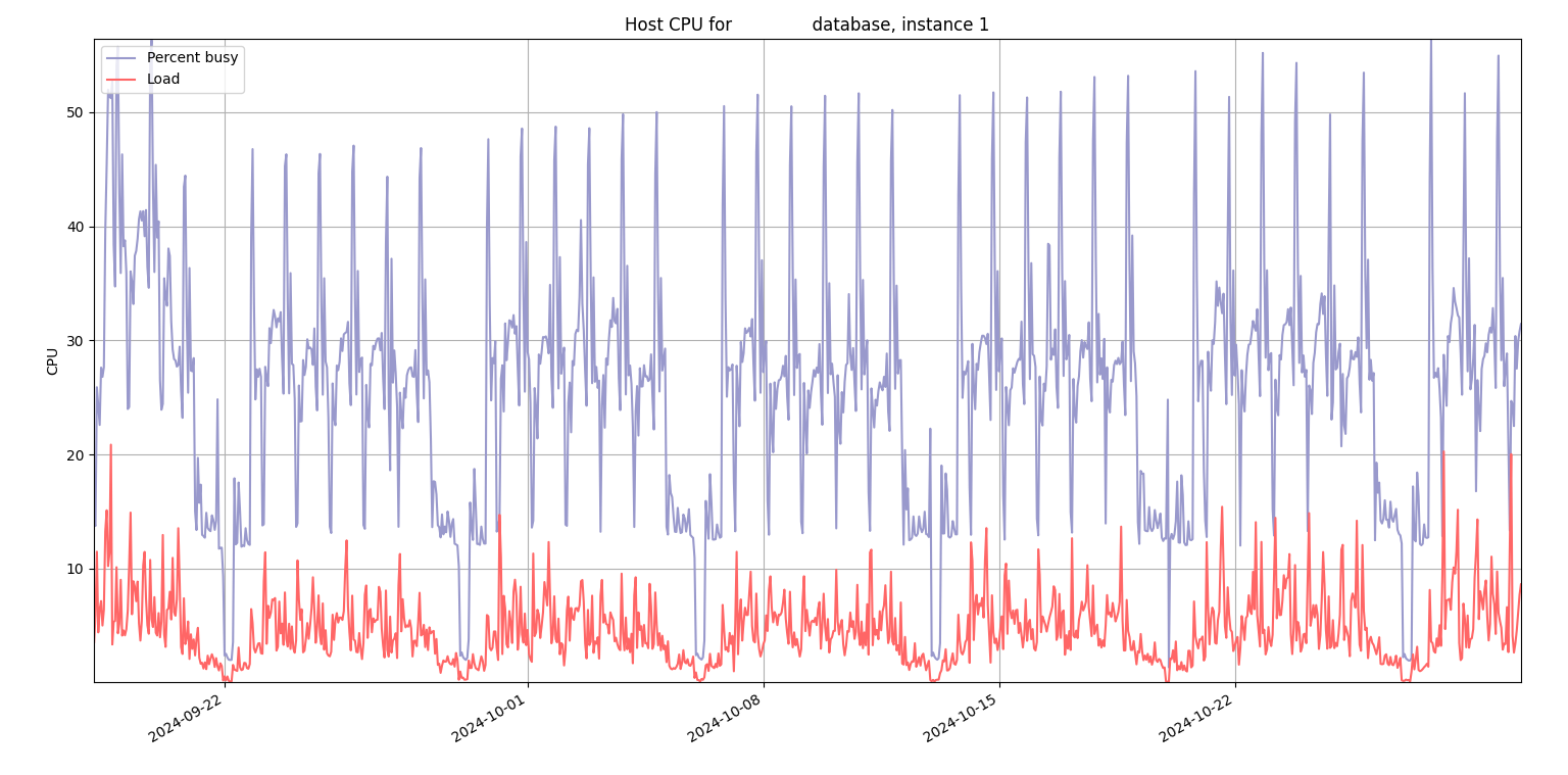
There is a relationship between the day of the week and the hour of the day and database performance metrics on many Oracle database systems. This is a graph from my hostcpu.py script that shows CPU utilization on a production Oracle database by date and hour of the day:

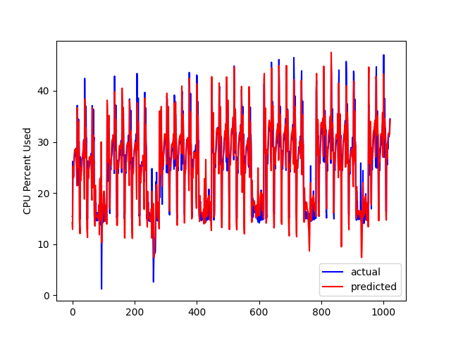
During the weekdays the CPU peaks at a certain hour and on the weekends, there are some valleys. So, I thought I would use PyTorch to model this relationship. Here is what the graph looks like of actual host CPU used versus predicted by PyTorch:

It’s the same source database but an earlier date. The prediction is close. I guess the big question after I got to this point was, so what? I’m not sure exactly what to do with it now that I have a model of the database CPU. I guess if the CPU is at 100% for an entire day instead of going up and down, I should throw an alert? What if CPU stays near 0% for a day during the week? It must be helpful to have a prediction of the host CPU but exactly how to alert on deviations from the predicted value is still a work in progress.

I thought it would be helpful to talk about the date and time inputs to this model. If you look at datetimeoscpu.sql in the zip it has this SQL for getting the date and time values:

select 
to_char(sn.END_INTERVAL_TIME,'D') day_of_week,
to_char(sn.END_INTERVAL_TIME,'DD') day_of_month,
to_char(sn.END_INTERVAL_TIME,'DDD') day_of_year,
to_char(sn.END_INTERVAL_TIME,'HH24') hour_of_day,
to_char(sn.END_INTERVAL_TIME,'MM') month,
to_char(sn.END_INTERVAL_TIME,'Q') quarter,
to_char(sn.END_INTERVAL_TIME,'WW') week_of_year,
to_char(sn.END_INTERVAL_TIME,'W') week_of_month,
to_char(sn.END_INTERVAL_TIME,'YYYY') year,
...

I ended up ignoring year because it is not a cyclical value. The rest have a range like 1 to 7 for day of week or 1 to 31 for day of month. Having all eight of these is probably overkill. I could just focus on day of week and hour of day and forget the other six. We have 6 weeks of AWR history so I’m not sure why I care about things like month, quarter, day of year because I don’t have multiple years of history to find a pattern.

My input data looks like this:

4 17 199 03 07 3 29 3 2024            15.4210261
4 17 199 04 07 3 29 3 2024            15.5799532
4 17 199 05 07 3 29 3 2024            26.2080227
4 17 199 06 07 3 29 3 2024            24.1532019
4 17 199 07 07 3 29 3 2024            23.2947767
4 17 199 08 07 3 29 3 2024            25.5198717
4 17 199 09 07 3 29 3 2024             26.029638
4 17 199 10 07 3 29 3 2024            27.1160204
4 17 199 11 07 3 29 3 2024            27.7076496

Each line represents an AWR snapshot. The first 8 are the cyclical date and time input values or X. The last value is the host CPU utilization percentage or Y. The point of the program is to create a model based on this data that will take in the 8 values and put out a predicted CPU percentage. This code was used to make the predictions for the graph at the end of the train.py script:

predictions = model(new_X)

When I first started working on this script it was not working well at all. I talked with ChatGPT about it and discovered that cyclical values like hour of day would work better with a PyTorch model if they were run through sine and cosine to transform them into the range -1 to 1. Otherwise PyTorch thinks that an hour like 23 is far apart from the hour 0 when really, they are adjacent. Evidently if you have both cosine and sine their different phases help the model use the cyclical date and time values. So, here is the code of the function which does sine and cosine:

def sinecosineone(dttmval,period):
    """
    Use both sine and cosine for each of the periodic
    date and time values like hour of day or
    day of month
    
    """
    # Convert dttmval to radians
    radians = (2 * np.pi * dttmval) / period
    # Apply sine and cosine transformations
    sin_dttmval = np.sin(radians)
    cos_dttmval = np.cos(radians)
    return sin_dttmval, cos_dttmval

def sinecosineall(X):
    """
    Column         Number
    
    day_of_week      7
    day_of_month     31
    day_of_year      366
    hour_of_day      24
    month            12
    quarter          4
    week_of_year     52
    week_of_month    5
    
    """
...

The period is how many are in the range – 24 for hour of the day. Here is the hour 23 and hour 0 example:

>>> sinecosineone(23.0,24.0)
(-0.25881904510252157, 0.9659258262890681)
>>> sinecosineone(0.0,24.0)
(0.0, 1.0)

Notice how the two values are close together for the two hours that are close in time. After running all my input data through these sine and cosine procedures they are all in the range -1.0 to 1.0 and these were fed into the model during training. Once I switched to this method of transforming the data the model suddenly became much better at predicting the CPU.

You can play with the scripts in the zip. I really hacked the Python script together based on code from ChatGPT, and I think one function from my class. It isn’t pretty. But you are welcome to it.

I’m starting to get excited about PyTorch. There are a bunch of things you must learn initially but the fundamental point seems simple. You start with a bunch of existing data and train a model that can be used as a function that maps the inputs to the outputs just as they were in the original data. This post was about an example of inputting cyclical date and time values like time of day or day of week and outputting performance metrics like CPU used percentage. I don’t have a perfect script that I have used to great results in production, but I am impressed by PyTorch’s ability to predict database server host CPU percent based on date and time values. More posts to come, but I thought I would get this out there even though it is imperfect. I hope that it is helpful.

Bobby