Bobby Durrett's DBA Blog

I’ve been working on testing performance on a database that uses Delphix as its storage system and ran across an unexpected side effect of using Delphix to clone a production database for testing.  Because Delphix uses NFS to present the filesystems for the datafiles you are required to use direct IO, at least on HP-UX which is our platform.  But, our production source database doesn’t have direct I/O turned on.  So, I’m seeing differences in runtimes in some queries that can be confusing if you don’t understand the reason.

If you have a query that uses direct path reads on a system that has a Unix filesystem and doesn’t use direct I/O those reads can be cached in the Unix filesystem’s buffer cache so that if you query that same table multiple times you eventually get direct path read times far lower than is possible on a system with direct I/O.  So, in our case if you have a developer running a test query on a non-Delphix, non-direct I/O system it can run many times faster than is possible on any system, Delphix or otherwise, that uses direct I/O.

This Oracle document spells out the requirements for using NFS for Oracle filesystems on various platforms:

Mount Options for Oracle files when used with NFS on NAS devices (Doc ID 359515.1)

For HP-UX datafiles you have to use:

rw,bg,vers=3,proto=tcp,noac,forcedirectio,hard,nointr,timeo=600,rsize=32768,wsize=32768,suid

Note the inclusion of “forcedirectio”.  This does just what it sounds like.  It forces the NFS filesystem to be accessed using direct I/O which bypasses the Unix filesystem buffer cache.  Generally direct I/O is the recommended option but when you implement Delphix you have a special situation.  The main point of Delphix is to be able to easily spin up multiple clones of your production database for development and testing.  This is great because it allows you to have a very realistic set of data to test against.  But, if your source system doesn’t use direct I/O you have introduced a difference from production that will affect testing.

I’ve put together a simple test case to show that direct path reads can be cached at the Unix filesystem level if you don’t have direct I/O and that with direct I/O – whether on a Delphix based NFS filesystem or a SAN based filesystem that uses direct I/O – you don’t see the effect of the Unix filesystem caching.  Here is the zip of the test case: zip.

I built a table big enough that 11 g Oracle would do direct path reads on a full scan:

create table test as select * from dba_objects where rownum < 1001;

insert /*+append */ into test select * from test;
commit;
insert /*+append */ into test select * from test;
commit;
insert /*+append */ into test select * from test;
commit;
insert /*+append */ into test select * from test;
commit;
insert /*+append */ into test select * from test;
commit;
insert /*+append */ into test select * from test;
commit;
insert /*+append */ into test select * from test;
commit;
insert /*+append */ into test select * from test;
commit;
insert /*+append */ into test select * from test;
commit;
insert /*+append */ into test select * from test;
commit;
insert /*+append */ into test select * from test;
commit;

execute dbms_stats.gather_table_stats(NULL,'TEST');

-- do an alter move to get blocks out of the buffer cache

alter table test move;

Then I ran a select against this table over and over again until I got the best results possible due to caching.  Here is what I got on a system (11.1.0.7) without direct I/O:

EVENT              AVERAGE_WAIT
------------------ ------------
direct path read              0

This is from v$session_event so the units are centiseconds rounded to the nearest hundredth centisecond.  So this means the direct path reads were averaging less than 100 microseconds so it must be cached at the database server host level.

Here is about the best I could get on our Delphix system:

EVENT             AVERAGE_WAIT
----------------- ------------
direct path read           .11

This is 1.1 milliseconds which means the data was probably cached within Delphix but not at the database server’s filesystem cache.

Just for comparison here is a SAN based filesystem with direct I/O and the same test:

EVENT              AVERAGE_WAIT
------------------ ------------
direct path read            .07

So, in every case with direct I/O we were stuck with around 1 millisecond or just under no matter how many times I ran the query to get things cached.  Without direct I/O it was about ten or more times faster.

Of course, not everything is going to be cached like this, especially large tables that you are doing full scans on and getting direct path I/O.  But there may be certain applications that run significantly different on your source system than on your target if your source is not using direct I/O, your target is using direct I/O, and your queries are doing direct path reads.

– Bobby

I haven’t figured out the best way to do this yet so this is a work in progress.  I’m trying to document the process of taking a large query that joins many tables together and breaking it into a series of small queries that only join two tables at a time.  Today I finished this process on a query that ran for four hours and the eleven queries I broke it up into together ran for five minutes.  I did put a full and use_hash hint on one of the eleven queries.

Here is the process I followed:

1. I started with permanent tables to save the intermediate results with the idea of making them global temporary tables with on commit preserve rows once I’d built all the new smaller queries.
2. I worked on one join at a time.  The query I worked on used the ANSI syntax for joins and had INNER and LEFT joins so I just worked in the order the tables were listed.
3. The first temp table was the output of joining the first two tables.  My query had twelve tables.  Every temp table after that was the result of joining the latest temp table T1…T10 to the next real table.
4. I included all of the columns in the select list and where clause from each real table I added to the join.  I’m sure there is a better way to to this.  Also, I took the table aliases like SLS and added them to the column names because there were columns of the same name from multiple tables.  I.e. PROD_CODE became SLS_PROD_CODE because there might be a PDT_PROD_CODE from the table with the alias PDT.
5. I inserted the final output into a table and compared it to the output from the original query to make sure they were exactly the same.

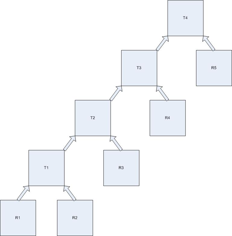
The weird thing about this in that there is no guarantee that  joining tables in the order listed in the query will produce good results, but in this case it was much faster than running the entire query.  It was kind of a one legged tree:

R1 through R5 represent my real tables from the original join.  Really there where twelve of these.

T1 through T4 represent the global temporaries created with each join.  In reality I had ten of these and the final output was inserted into a permanent table.

I don’t really know why breaking the query up into these small pieces was so effective but I do know that it would have taken a lot more work to try to make the bigger query run faster.  It took time to split it up but it wasn’t difficult if you know what I mean.  I was just tedious getting the list of column names edited together but that’s a lot easier than figuring out why the query with twelve tables joined together was taking four hours to run.

– Bobby

I had a situation today where I had two slightly different queries that I thought should have the same plan but they didn’t.  So, I needed a way to force the slower query to run with the same plan as the faster one.  I wanted to do this so I could see if the row counts, bytes, or costs for the second query would be different than on the first.  Something must be different or the optimizer would have chosen the same plan for both queries.  By imposing the fast query’s plan on the slow one I could see where the optimizer’s calculations are different.

In the past I’ve done this by adding hints such as an INDEX hint if the faster one used an index and the slower one didn’t.  Today the query was pretty complex so I used an outline hint to force all aspects of the plan on the slow query to be the same as the fast one.  I’ve put together a simplistic example of how to do this.  Script and log is in this zip.

My fast query example is hinted to use an index just to make it different from my slow example:

SQL> -- Get plan for query with index hint including outline
SQL> 
SQL> explain plan into plan_table for
  2  select /*+index(test testi) */ * from test
  3  /

Explained.

SQL> 
SQL> select * from table(dbms_xplan.display('PLAN_TABLE',NULL,
'OUTLINE'));

PLAN_TABLE_OUTPUT
-------------------------------------------------------------------
Plan hash value: 2400950076

--------------------------------------------------------------------
| Id  | Operation                   | Name  | Rows  | Bytes | Cost  
--------------------------------------------------------------------
|   0 | SELECT STATEMENT            |       | 31471 |  7191K|  1190 
|   1 |  TABLE ACCESS BY INDEX ROWID| TEST  | 31471 |  7191K|  1190 
|   2 |   INDEX FULL SCAN           | TESTI | 31471 |       |    80 
--------------------------------------------------------------------

Outline Data
-------------

  /*+
      BEGIN_OUTLINE_DATA
      INDEX(@"SEL$1" "TEST"@"SEL$1" ("TEST"."OWNER"))
      OUTLINE_LEAF(@"SEL$1")
      ALL_ROWS
      OPT_PARAM('_unnest_subquery' 'false')
      DB_VERSION('11.2.0.3')
      OPTIMIZER_FEATURES_ENABLE('11.2.0.3')
      IGNORE_OPTIM_EMBEDDED_HINTS
      END_OUTLINE_DATA
  */

It’s not a realistic example.  The index version of this plan is really slower.  But pretend you wanted to force a similar query to use the same plan as this first query.

Here is the second query with no hints:

SQL> -- Get plan for query with no hint
SQL> 
SQL> explain plan into plan_table for
  2  select * from test
  3  /

Explained.

SQL> select * from table(dbms_xplan.display('PLAN_TABLE',NULL,
'BASIC'));

PLAN_TABLE_OUTPUT
-------------------------------------
Plan hash value: 217508114

----------------------------------
| Id  | Operation         | Name |
----------------------------------
|   0 | SELECT STATEMENT  |      |
|   1 |  TABLE ACCESS FULL| TEST |
----------------------------------

Now here is the second query with the outline hint added and its resulting plan – same as the first query’s:

SQL> -- Get plan forcing query using outline
SQL> 
SQL> explain plan into plan_table for
  2  select
  3    /*+
  4        BEGIN_OUTLINE_DATA
  5        INDEX(@"SEL$1" "TEST"@"SEL$1" ("TEST"."OWNER"))
  6        OUTLINE_LEAF(@"SEL$1")
  7        ALL_ROWS
  8        OPT_PARAM('_unnest_subquery' 'false')
  9        DB_VERSION('11.2.0.3')
 10        OPTIMIZER_FEATURES_ENABLE('11.2.0.3')
 11        IGNORE_OPTIM_EMBEDDED_HINTS
 12        END_OUTLINE_DATA
 13    */
 14  * from test
 15  /

Explained.

SQL> 
SQL> select * from table(dbms_xplan.display('PLAN_TABLE',NULL,
'BASIC'));

PLAN_TABLE_OUTPUT
------------------------------------------------
Plan hash value: 2400950076

---------------------------------------------
| Id  | Operation                   | Name  |
---------------------------------------------
|   0 | SELECT STATEMENT            |       |
|   1 |  TABLE ACCESS BY INDEX ROWID| TEST  |
|   2 |   INDEX FULL SCAN           | TESTI |
---------------------------------------------

So, imagine a scenario where the two queries were similar enough to have the same plan but complex enough that figuring out individual hints to force the second one to have the same plan as the first would take some time.  This outline hint method is an easy way to impose the first query’s plan on the second.  It won’t work if the two queries are too different but today I used this in a real tuning situation and it saved me a lot of time.

– Bobby

Most recent version here(updated).

Added these two:

display_results(test_name,compared_to_test_name) - output results of
testings in the two scenarios.  List results from all queries that
ran more than 3 times as long with one test or the other.  Also 
summarize results with total elapsed time, number of queries 
executed, average elapsed time, and percent improvement.

show_plan(test_name,sqlnumber) - extract plan from plan_table for
given test name and sql statement.

Example usage:

execute test_select.display_results('PARALLEL 128','PARALLEL 8');

select test_select.show_plan('PARALLEL 128',57) from dual;

Give it a try.

– Bobby

Quick update to package from previous post.

Here is the zip of the download: zip(updated)

I added these procs to collect select statements on a source production database and to copy them back (as clobs) to the test database:

collect_select_statements(max_number_selects,
include_pattern1,...,include_pattern10,
exclude_pattern1,...,exclude_pattern10)

This proc is run on the the source database to 
collect select statements including statements 
that have the include patterns and excluding those 
who have the exclude patterns. 

Patterns use LIKE conditions %x%.

copy_select_statements(link_name)

copies select statements from remote source 
database pointed to by link_name's db link.

I intended to have this functionality in the package from the beginning but I got bogged down getting ORA-22992 errors trying to copy a clob from a remote table into a variable.  So, now I just execute collect_select_statements on the remote database over the link and run copy_select_statements to copy the populated table back to the test database:

execute TEST_SELECT.
collect_select_statements@myqalink
(10,include_pattern1=>'%TARGETTABLE%');

execute TEST_SELECT.
copy_select_statements('myqalink');

I’ve uploaded this package(updated) that I’m using to test some large select statements.  See the file packagedescriptionv1.txt for a description of the package.  Also, test.sql and test.log is an example of using the package.

This is an updated version of the scripts in this post.

– Bobby

This weekend we had the most convincing evidence that our change from dedicated to shared servers on a database that supports a farm of web servers was the right move.  We have had some outages on the weekend caused by a sudden burst in web server generated database activity.  In the past the CPU load would spike and log file sync (commit) waits would be 20 times slower and we would have to bounce the database and web servers to recover.  Sunday we had a similar spike in database activity without having any sort of outage.

Here is a section of the AWR report from the last weekend outage:

Top 5 Timed Events

Here is the same part of the AWR report for this weekend’s spike in activity:

Top 5 Timed Events

These are hour long intervals, in both cases between 9 and 10 am central on the first Sunday of a Month (June and August).  The key is that in both cases there are around 600,000 commits in that hour.  During the outage in June the commits took 247 milliseconds, a quarter of a second, each.  This Sunday they took only 11 milliseconds.  Note that in both cases the disk IO for commits – log file parallel write – was only 2 milliseconds.  So, the difference was CPU and primarily queuing for the CPU.  So, with dedicated servers we had 20 times as much queuing for the CPU roughly (247 ms/11 ms).  Note that during our normal peak processing log file sync is 3 milliseconds so even the 11 milliseconds we saw this weekend represents some queuing.

The key to this is that we have the number of shared server processes set to twice the number of CPUs.  When I say “CPUs” I mean from the Unix perspective.  They are probably cores, etc. But, Unix thinks we have 16 CPUs.  We have 32 shared server processes.  This prevents CPU queuing because even if all 32 shared servers are running full out they probably wont max out the CPU because they will be doing things besides CPU some of the time.  The ideal number may not be 2x CPUs.  It may be 1.5 or 2.3 but the point is there is some number of shared server processes that under overwhelming load will allow the CPU to be busy but not allow a huge queue for the CPU.  Two times the number of CPUs is a good starting point and this was what Tom Kyte recommended in my ten minute conversation with him that spawned this change to shared servers.

With dedicated servers we would have hundreds of processes and they could easily max out the CPU and then the log writer process(LGRW) would split time waiting on the CPU equally with the hundreds of active dedicated server processes.  I think what was really happening with dedicated servers is that hundreds of sessions were hung up waiting on commits and then the session pools from the web servers started spawning new connections which themselves ate up CPU and a downward spiral would occur that we could not recover from.  With shared servers the commits remained efficient and the web servers didn’t need to spawn so many new connections because they weren’t hung up waiting on commits.

If you are supporting a database that has a lot of web server connections doing a lot of commits you might want to consider shared servers as an option to prevent the log writer from being starved for CPU.

Here are my previous posts related to this issue for reference:

 https://www.bobbydurrettdba.com/2013/07/19/shared-servers-results-in-lower-cpu-usage-for-top-query-in-awr/

https://www.bobbydurrettdba.com/2013/06/26/testing-maximum-number-of-oracle-sessions-supported-by-shared-servers/

https://www.bobbydurrettdba.com/2012/08/30/faster-commit-time-with-shared-servers/

https://www.bobbydurrettdba.com/2012/03/21/reducing-size-of-connection-pool-to-improve-web-application-performance/

It may be tough to convince people to move to shared servers since it isn’t a commonly used feature of the Oracle database but in the case of hundreds of sessions with lots of commits it makes sense as a way of keeping the commit process efficient.

– Bobby

P.S.  Here are our parameters in production related to the shared servers change with the ip address removed.  We had to bump up the large pool and set local_listener in addition to setting the shared servers and dispatchers parameters.  I added newlines to the dispatchers and local listener parameters to fit on this page.

NAME                                 VALUE
------------------------------------ -------------------
max_shared_servers                   32
shared_servers                       32
dispatchers                          (PROTOCOL=TCP)
                                     (DISPATCHERS=64)
max_dispatchers                      
local_listener                       (ADDRESS=
                                     (PROTOCOL=TCP)
                                     (HOST=EDITEDOUT)
                                     (PORT=1521))
large_pool_size                      2G

P.P.S.  This server is on HP-UX 11.11 and Oracle 10.2.0.3.

I’m trying to test some select statements that have some lines longer than 4000 characters and I couldn’t get them to run in sqlplus so I built this proc to run a select statement that is stored in a CLOB and return the number of rows fetched and elapsed time in seconds.

CREATE OR REPLACE procedure runclob(
       sqlclob  in clob,
       total_rows_fetched out NUMBER,
       elapsed_time_seconds out NUMBER) is
    clob_cursor INTEGER;
    rows_fetched INTEGER;
    before_date date;
    after_date date;
BEGIN
    select sysdate into before_date from dual;

    clob_cursor := DBMS_SQL.OPEN_CURSOR;

    DBMS_SQL.PARSE (clob_cursor,sqlclob,DBMS_SQL.NATIVE);

    rows_fetched := DBMS_SQL.EXECUTE_AND_FETCH (clob_cursor);
    total_rows_fetched := rows_fetched;

    LOOP
        EXIT WHEN rows_fetched < 1;
        rows_fetched := DBMS_SQL.FETCH_ROWS (clob_cursor);
        total_rows_fetched := total_rows_fetched + rows_fetched;
    END LOOP;

    DBMS_SQL.CLOSE_CURSOR (clob_cursor);

    select sysdate into after_date from dual;

    elapsed_time_seconds := (after_date-before_date)*24*3600;
END;
/

The queries I’m working on are generated by OBIEE and I’m testing running them with two different optimizer statistics choices and I want to see which causes a group of queries to run faster.  I will have a block of code that loops through a collection of select statements that I extracted from production and runs each one in my test database with the proc listed above.

– Bobby

One of our senior developers found a way to greatly improve the performance of a query by adding a dynamic sampling hint for a table that had multiple correlated conditions in its where clause.  This led me to try to understand why the dynamic sampling hint helped and it appears that a dynamic sampling hint can deal with correlated predicates in the where clause better than multi-column histograms.

A quick Google search about the dynamic sampling hint found this article by Tom Kyte.  The section titled “When the Optimizer Guesses” seemed to match the symptoms I saw in the query our developer was tuning.  So, I started messing with the test case from the article and found that multi-column histograms would not make the test case run the efficient plan with the index scan but dynamic sampling, even at level 1, would.

I used the following commands to gather stats:

select DBMS_STATS.CREATE_EXTENDED_STATS (NULL,'T','(FLAG1,FLAG2)') from dual;
execute DBMS_STATS.GATHER_TABLE_STATS (NULL,'T',estimate_percent=>NULL,method_opt=>'FOR ALL COLUMNS SIZE 254');

Here is the plan without the dynamic sampling hint:

Execution Plan
----------------------------------------------------------
Plan hash value: 2153619298

--------------------------------------------------------------------------
| Id  | Operation         | Name | Rows  | Bytes | Cost (%CPU)| Time     |
--------------------------------------------------------------------------
|   0 | SELECT STATEMENT  |      | 37371 |  3941K|   580   (1)| 00:00:07 |
|*  1 |  TABLE ACCESS FULL| T    | 37371 |  3941K|   580   (1)| 00:00:07 |
--------------------------------------------------------------------------

Predicate Information (identified by operation id):
---------------------------------------------------

   1 - filter("FLAG1"='N' AND "FLAG2"='N')

Here is the plan with this hint: dynamic_sampling(t 1)

Execution Plan
----------------------------------------------------------
Plan hash value: 1020776977

-------------------------------------------------------------------------------------
| Id  | Operation                   | Name  | Rows  | Bytes | Cost (%CPU)| Time     |
-------------------------------------------------------------------------------------
|   0 | SELECT STATEMENT            |       |    54 |  5832 |     3   (0)| 00:00:01 |
|   1 |  TABLE ACCESS BY INDEX ROWID| T     |    54 |  5832 |     3   (0)| 00:00:01 |
|*  2 |   INDEX RANGE SCAN          | T_IDX |    54 |       |     1   (0)| 00:00:01 |
-------------------------------------------------------------------------------------

Predicate Information (identified by operation id):
---------------------------------------------------

   2 - access("FLAG1"='N' AND "FLAG2"='N')

Note
-----
   - dynamic sampling used for this statement (level=2)

If you look at a 10053 trace you see that dynamic sampling is running this query:

SELECT
...bunch of hints edited out...
NVL (SUM (C1), 0), NVL (SUM (C2), 0), NVL (SUM (C3), 0)
  FROM (SELECT /*+ ...more hints... */
              1 AS C1,
               CASE
                  WHEN "T"."FLAG1" = 'N' AND "T"."FLAG2" = 'N' 
                  THEN 1
                  ELSE 0
               END
                  AS C2,
               CASE
                  WHEN "T"."FLAG2" = 'N' AND "T"."FLAG1" = 'N' 
                  THEN 1
                  ELSE 0
               END
                  AS C3
          FROM "MYUSERID"."T" SAMPLE BLOCK (0.519350, 1) 
               SEED (1) "T") SAMPLESUB

I think this is the same query that is in the article but in the 10053 trace it is easier to see the constants “T”.”FLAG2″ = ‘N’ AND “T”.”FLAG1″ = ‘N’.  So, it shows that dynamic sampling is running a query with the where clause conditions.  In the 10053 trace for our production query the dynamic sampling query came back with all of the conditions on the table that we hinted.

Note that if you leave stats off of the table you get the same good plan:

Execution Plan
----------------------------------------------------------
Plan hash value: 1020776977

-------------------------------------------------------------------------------------
| Id  | Operation                   | Name  | Rows  | Bytes | Cost (%CPU)| Time     |
-------------------------------------------------------------------------------------
|   0 | SELECT STATEMENT            |       |     1 |   162 |     1   (0)| 00:00:01 |
|   1 |  TABLE ACCESS BY INDEX ROWID| T     |     1 |   162 |     1   (0)| 00:00:01 |
|*  2 |   INDEX RANGE SCAN          | T_IDX |     1 |       |     1   (0)| 00:00:01 |
-------------------------------------------------------------------------------------

Predicate Information (identified by operation id):
---------------------------------------------------

   2 - access("FLAG1"='N' AND "FLAG2"='N')

Note
-----
   - dynamic sampling used for this statement (level=2)

So, with no stats on the table it must be doing the same dynamic sampling query with all the where clause conditions.

Interestingly, in the case of the real query the table is very small.  I’m thinking we need to just delete the stats from the table and lock them empty.  That way every query with the table will dynamically sample the small table and handle correlated predicates better than multi-column stats.

Here is my test script and its log.

– Bobby

So, this isn’t really Oracle related except that I got a new Windows 7 laptop to support Oracle and I’m getting an annoying popup message every time I try to run putty to access a database server.

I looked up the message “The publisher could not be verified” and Windows 7 and found a bunch of stuff about changing Windows policies or internet security – yuck!  I found a simpler solution.

I have putty.exe installed in c:\putty on my laptop.  I added a bat file called putty.bat in c:\putty that has these lines in it:

start /b c:\putty\putty.exe

Then I created a shortcut on my desktop to run c:\putty\putty.bat but to start the command prompt window minimized:

Now when I click on this shortcut putty pops right up without the publisher could not be verified message.

– Bobby