
1. Introduction
I set out to use Machine Learning to monitor Oracle databases but ultimately chose not to. The most valuable lesson I learned was the importance of visualizing my data to determine the best approach. By examining real production performance issues, I developed scripts that trigger alerts during potential performance problems. I used six weeks of historical performance metrics to compare current behavior against past trends. I already knew that a high value for a given metric didn’t necessarily indicate a performance issue with business impact. In the end, I built a script that sends an alert when certain metrics are the top wait event and are performing three times worse than at any point in the past six weeks. While it doesn’t guarantee a business impact, it flags anomalies that are unusual enough to warrant investigation.
2. Why I Tried Machine Learning
I think anyone reading this post would know why I tried to use Machine Learning. It’s very popular now. I took a class online about ML with Python and I bought a book about the same subject. I had already used Python in some earlier classes and in my work, so it was natural to take a class/read a book about ML based on Python. As I mentioned in an earlier post, I studied AI in school many years ago and there have been many recent advances so naturally I wanted to catch up with the current state of the art in AI and ML. Having taken the class, and later having read a book, I needed some application of what I learned to a valuable business problem. We had a couple of bad performance problems with our Oracle databases and our current monitoring didn’t catch them. So, I wanted to use ML – specifically with PyTorch in a Python script – to write a script that would have alerted on those performance problems.
3. Failed Attempt Number One – Autoencoder
In my first attempt to write a monitoring script, I worked with Copilot and ChatGPT to hack together a script using an autoencoder model. I queried a bunch of our databases and collected a list of all the wait events. My idea was to treat each wait as an input to the autoencoder. For each wait, I pulled the number of events and the total wait time over the past hour. I didn’t differentiate between foreground and background waits—I figured AI could sort that out. I also included DB time and DB CPU time. These were all deltas between two hourly snapshots, so the data represented CPU and waits for a given hour.
The concept behind the autoencoder was to compress these inputs into a smaller set of values and then reconstruct the original inputs. With six weeks of hourly snapshots, I trained the autoencoder on that historical data, assuming it represented “normal” behavior. The idea was that any new snapshot that couldn’t be accurately reconstructed by the model would be considered abnormal and trigger an alert.
I got the model fully running across more than 20 production databases. I tuned the threshold so it would have caught two recent known performance issues. But in practice, it didn’t work well. It mostly triggered alerts on weekends when backups were running and I/O times naturally spiked. It wasn’t catching real performance problems—it was just reacting to predictable noise.
Here is the PyTorch autoencoder model:
# Define the Autoencoder model
class TabularAutoencoder(nn.Module):
    def __init__(self, input_dim):
        super(TabularAutoencoder, self).__init__()
        # Encoder
        self.encoder = nn.Sequential(
            nn.Linear(input_dim, 64),  # Reduce dimensionality from input_dim to 64
            #nn.LayerNorm(64),  # Layer Normalization for stability
            nn.ReLU(True),
            nn.Dropout(0.2),   # Dropout for regularization
            nn.Linear(64, 32),  # Reduce to 32 dimensions
            nn.ReLU(True),
            nn.Linear(32, 16),  # Bottleneck layer (compressing to 16 dimensions)
        )
        # Decoder
        self.decoder = nn.Sequential(
            nn.Linear(16, 32),  # Expand back to 32 dimensions
            nn.ReLU(True),
            nn.Linear(32, 64),  # Expand to 64 dimensions
            #nn.LayerNorm(64),  # Layer Normalization for stability
            nn.ReLU(True),
            nn.Linear(64, input_dim),  # Expand back to original input dimension
         )

    def forward(self, x):
        x = self.encoder(x)
        x = self.decoder(x)
        return x
4. Failed Attempt Number Two – Binary Classification
Much more recently, I came back to using a PyTorch model to build an alerting script. I had spent some time learning about large language models and exploring how to apply GenAI to business problems, rather than working with these simpler ML models in PyTorch. But I decided to give it another try and see if I could fix the limitations I ran into with the autoencoder approach.
I didn’t really expect binary classification to work, but it’s the simplest kind of ML model, so I thought it was worth a shot. I selected a few snapshots that occurred during a severe performance problem on an important Oracle database. I labeled these as 1 (problem), and the rest as 0 (no problem). It was easy enough to train a model that correctly identified the problem snapshots during training and testing.
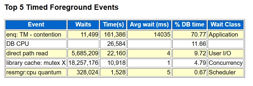
However, when I applied the model to later snapshots it hadn’t seen before, it started generating false alarms that didn’t make sense. It got even worse when I tried it on a completely different database. I had expected the model to pick up on the fact that the top wait event during the problem period was enq: TM – contention. A quick glance at the top foreground events in an AWR report made it obvious that this was the issue. But the trained model ended up sending an alert on snapshots that didn’t even have this wait event in the top waits.
Here is the PyTorch binary classification model:
"""

Mostly got the model from Copilot. input_dim is the number of performance
metrics which is over 100. Gets it down to 64 to 32 and then 1.
The ReLU functions add "non-linear" change to allow it to do
functions that the linear steps can't do.

"""

class MyModel(nn.Module):
    def __init__(self, input_dim):
        super(MyModel, self).__init__()
        self.fc1 = nn.Linear(input_dim, 64)
        self.relu1 = nn.ReLU()
        self.fc2 = nn.Linear(64, 32)
        self.relu2 = nn.ReLU()
        self.output = nn.Linear(32, 1)

    def forward(self, x):
        x = self.fc1(x)
        x = self.relu1(x)
        x = self.fc2(x)
        x = self.relu2(x)
        x = self.output(x)
        return x
Here are the foreground waits and cpu from an AWR report of the problem time:
5. Failed Attempt Number Three – Z-Score
While talking with Copilot, I decided to try a simple statistical approach to anomaly detection. One suggestion was to use a z-score. In my context, this meant looking at the top foreground wait event—enq: TM – contention—in the current snapshot and calculating its z-score relative to the mean and standard deviation of that wait’s values in previous snapshots.
Like the binary classification attempt, the z-score alerting script worked well with the original snapshots from the known problem period. But when I ran the same script against other databases, it produced a lot of false alarms.
Output of z-score script on problem database (alerts on expected snapshot):
   SNAP_ID SNAP_DTTIME         EVENT_NAME            RATIO_ZSCORE AVGWAIT_ZSCORE
---------- ------------------- --------------------- ------------ --------------
    151752 2025-06-19 00:00:41 enq: TM - contention     3.0878532     9.74301378
Output on another database (no rows expected):
   SNAP_ID SNAP_DTTIME         EVENT_NAME                    RATIO_ZSCORE AVGWAIT_ZSCORE
---------- ------------------- ----------------------------- ------------ --------------
     48916 2025-06-22 01:00:01 cursor: pin S wait on X         9.00654128     5.36254393
     48917 2025-06-22 02:00:06 cursor: pin S wait on X         7.16211659     8.09929239
     48918 2025-06-22 03:00:11 cursor: pin S wait on X         5.41578347     4.52106805
     48919 2025-06-22 04:00:13 cursor: pin S wait on X         4.69593403     4.08335551
     48920 2025-06-22 05:00:16 cursor: pin S wait on X         3.17592316     3.46979661
     49081 2025-06-28 22:00:32 cursor: pin S wait on X         4.62636243     3.15122436
     49254 2025-07-06 03:00:04 cursor: pin S wait on X         4.73771834     3.23654318
     49255 2025-07-06 04:00:10 cursor: pin S wait on X         3.96208561     3.61732606
     49289 2025-07-07 14:00:55 SQL*Net more data from dblink   18.2249941     6.61795927
     49364 2025-07-10 17:00:20 library cache lock              89.7469665     392.322777
     49365 2025-07-10 18:00:45 library cache lock              14.6228987      120.71596
     49760 2025-07-27 05:00:21 cursor: pin S wait on X         5.68469758     3.52381292
6. A Picture Is Worth a Thousand Words
Now I’m getting to the high point of this post. I graphed the waits for the snapshots where the z-score worked and the ones where it didn’t—and the truth jumped out at me. In the database with the known problem, the graph of enq: TM – contention was almost a flat line across the bottom for six weeks, followed by a huge spike during the problem hours. In another database—or even the same one with a different top wait—the graph looked completely different: a wavy pattern, almost like a sine wave, stretching back across the entire six weeks.
“Heck!” I said to myself. “Why don’t I just look for top waits that are never close to this high in the past six weeks?” Sure, it might not always be a real business problem, but if a wait is so dramatically different from six weeks of history, it’s worth at least sending an email—if not a wake-up-in-the-middle-of-the-night page.
With z-score, we were sending an alert when a metric was three standard deviations from the mean. But for wavy waits like db file sequential read, that wasn’t selective enough. So, I designed a new monitoring script: it looks at the top wait in the snapshot, checks if it’s a higher percentage of DB time than CPU, and then compares it to the past six weeks. If it’s more than three times higher than it’s ever been in that history, it triggers an alert. This is all based on the percentage of total DB time.
First the wavy graph of db file sequential read waits:
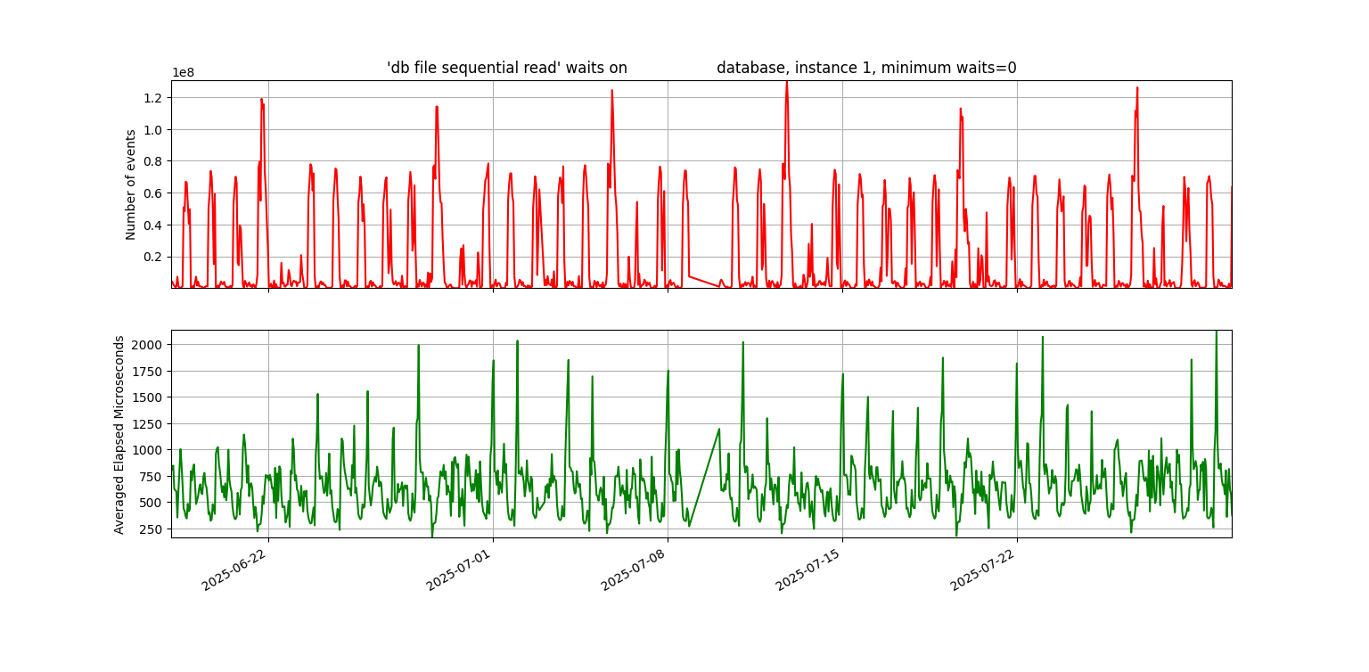
Next, this is the key graph to this entire post. Not wavy:
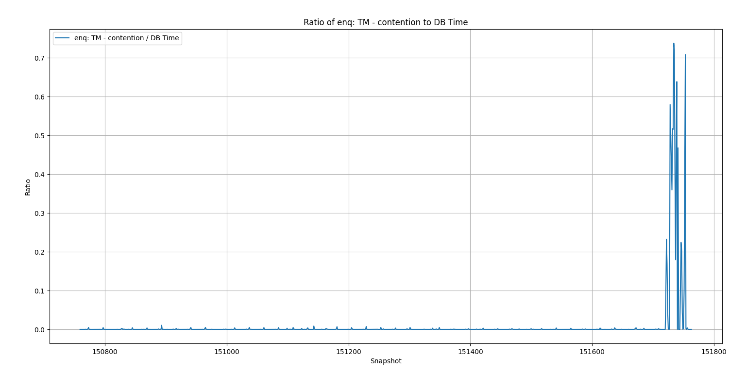
The light clicked on when I saw this graph. The enq: TM – contention waits were insignificant until the problem occurred.
Here is the script that checks if we should alert: neveralert.sql
7. Don’t Check Your Brain at the Machine Learning Door
When I started with the autoencoder script, I felt overwhelmed—like many people do when first approaching Artificial Intelligence and Machine Learning. I expected the model to magically work without fully understanding how or why. I relied on chat tools to help me piece together code I didn’t grasp, and when it didn’t work, I couldn’t explain why. I’m trying to be honest about my journey here so it might help others and remind myself what I learned.
Each step—from binary classification to z-score to manual logic—brought me closer to a solution rooted in my own experience. You must use your own brain. This has always been true in Oracle performance work: you can’t just follow something you read or heard about without understanding it. You need to think critically and apply your domain knowledge.
If it sounds like I didn’t get anything out of my machine learning training, that’s not the case. Both the class and the book emphasized the importance of visualizing data to guide modeling decisions. They used Matplotlib to create insightful graphs, and while I’ve used simpler visualizations in my own PythonDBAGraphs repo, this experience showed me the value of going deeper with data visualization. I think both the class and book would agree: visualizing your data is one of the best ways to decide how to use it.
Even though this journey didn’t end with a PyTorch-based ML solution, it sharpened my understanding of both ML and Oracle performance—and I’m confident it will help me build better solutions in the future.
Bobby

Very interesting, Bobby!
Thanks Karl! I hope that you and your family are doing well. I’m trying to get up to speed on some of the new AI technology while still doing my regular database tasks. It’s interesting but challenging.